III.43 Jordan Normal Form

Suppose that you are presented with an n × n real or complex MATRIX [I.3 §4.2] A and would like to understand it. You might ask how it behaves as a LINEAR MAP [I.3 §4.2] on ⁿ or ⁿ, or you might wish to know what the powers of A are. In general, answering these questions is not particularly easy, but for some matrices it is very easy. For example, if A is a diagonal matrix (that is, one whose nonzero entries all lie on the diagonal), then both questions can be answered immediately: if x is a vector in ⁿ or ⁿ, then Ax will be the vector obtained by multiplying each entry of x by the corresponding diagonal element of A, and to compute A^m you just raise each diagonal entry to the power m.

So, given a linear map T (from ⁿ to ⁿ or from ⁿ to ⁿ), it is very nice if we can find a basis with respect to which T has a diagonal matrix; if this can be done, then we feel that we “understand” the linear map. Saying that such a basis exists is the same as saying that there is a basis consisting of EIGENVECTORS [I.3 §4.3]: a linear map is called diagonalizable if it has such a basis. Of course, we may apply the same terminology to a matrix (since a matrix A determines a linear map on ⁿ or ⁿ, by mapping x to Ax). So a matrix is also called diagonalizable if it has a basis of eigenvectors, or equivalently if there is an invertible matrix P such that P^-1 AP is diagonal.

Is every matrix diagonalizable? Over the reals, the answer is no for uninteresting reasons, since there need not even be any eigenvectors: for example, a rotation in the plane clearly has no eigenvectors. So let us restrict our attention to matrices and linear maps over the complex numbers.

If we have a matrix A, then its characteristic polynomial, namely det(A - tI), certainly has a root, by THE FUNDAMENTAL THEOREM OF ALGEBRA [V.13]. If is such a root, then standard facts from linear algebra tell us that A - I is singular, and therefore that there is a vector x such that (A - I)x = 0, or equivalently that Ax = x. So we do have at least one eigenvector. Unfortunately, however, there need not be enough eigenvectors to form a basis. For example, consider the linear map T that sends (1, 0) to (0, 1) and (0, 1) to (0, 0). The matrix of this map (with respect to the obvious basis) is . This matrix is not diagonalizable. One way of seeing why not is the following. The characteristic polynomial turns out to be t², of which the only root is 0. An easy computation reveals that if Ax = 0 then x has to be a multiple of (0, 1), so we cannot find two linearly independent eigenvectors. A rather more elegant method of proof is to observe that T² is the zero matrix (since it maps each of (1, 0) and (0, 1) to (0, 0)), so that if T were diagonalizable, then its diagonal matrix would have to be zero (since any nonzero diagonal matrix has a nonzero square), and therefore T would have to be the zero matrix, which it is not.

The same argument shows that any matrix A such that A^k = 0 for some k (such matrices are called nilpotent) must fail to be diagonalizable, unless A is itself the zero matrix. This applies, for example, to any matrix that has all of its nonzero entries below the main diagonal.

What, then, can we say about our nondiagonalizable matrix T above? In a sense, one feels that (1, 0) is “nearly” an eigenvector, since we do have T²(1, 0) = (0, 0). So what happens if we extend our point of view by allowing such vectors? One would say that a vector x is a generalized eigenvector of T, with eigenvalue , if some power of T - maps x to zero. For instance, in our example above the vector (1, 0) is a generalized eigenvector with eigenvalue 0. And, just as we have an “eigenspace” associated with each eigenvalue (defined to be the space of all eigenvectors with eigenvalue ), we also have a “generalized eigenspace”, which consists of all generalized eigenvectors with eigenvalue .

Diagonalizing a matrix corresponds exactly to decomposing the vector space (ⁿ) into eigenspices. So it is natural to hope that one could decompose the vector space into generalized eigenspaces for any matrix. And this turns out to be true. The way of breaking up the space is called Jordan normal form, which we shall now describe in more detail.

Let us pause for a moment and ask: what is the very simplest situation in which we get a generalized eigenvector? It would surely be the obvious generalization of the above example to n dimensions. In other words, we have a linear map T that sends e₁ to e₂, e₂ to e₃, and so on, until e_n-1 is sent to e_n , with e_n itself mapped to zero. This corresponds to the matrix

Although this matrix is not diagonalizable, its behavior is at least very easy to understand.

The Jordan normal form of a matrix will be a diagonal sum of matrices that are easily understood in the way that this one is. Of course, we have to consider eigenvalues other than zero: accordingly, we define a block to be any matrix of the form

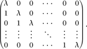
Note that this matrix A, with I subtracted, is precisely the matrix above, so that (A- I)ⁿ is indeed zero. Thus, a block represents a linear map that is indeed easy to understand, and all its vectors are generalized eigenvectors with the same eigenvalue. The Jordan normal form theorem tells us that every matrix can be decomposed into such blocks: that is, a matrix is in Jordan normal form if it is of the form

Here, the B_i are blocks, which can have different sizes, and the 0s represent submatrices of the matrix with sizes depending on the block sizes. Note that a block of size 1 simply consists of an eigenvector.

Once a matrix A is put into Jordan normal form, we have broken up the space into subspaces on which it is easy to understand the action of A. For example, suppose that A is the matrix

which is made out of three blocks, of sizes 3, 2, and 2. Then we can instantly read off a great deal of information about A. For instance, consider the eigenvalue 4. Its algebraic multiplicity (its multiplicity as a root of the characteristic polynomial) is 5, since it is the sum of the sizes of all the blocks with eigenvalue 4, while its geometric multiplicity (the dimension of its eigenspace) is 2, since it is the number of such blocks (because in each block we only have one actual eigenvector). And even the minimal polynomial of the matrix (the smallest-degree polynomial P(t) such that P(A) = 0) is easy to write down. The minimal polynomial of each block can be written down instantly: if the block has size k and generalized eigenvalue , then it is (t - )^k. The minimal polynomial of the whole matrix is then the “lowest common multiple” of the polynomials for the individual blocks. For the matrix above, we get (t - 4)³, (t - 4)², and (t - 2)² for the three blocks, so the minimal polynomial of the whole matrix is (t -4)³ (t - 2)².

There are some generalizations of Jordan normal form, away from the context of linear maps acting on vector spaces. For example, there is an analogue of the theorem that applies to Abelian groups, which turns out to be the statement that every finite Abelian group can be decomposed as a direct product of cyclic groups.