III.17 Dimension

What is the difference between a two-dimensional set and a three-dimensional set? A rough answer that one might give is that a two-dimensional set lives inside a plane, while a three-dimensional set fills up a portion of space. Is this a good answer? For many sets it does seem to be: triangles, squares, and circles can be drawn in a plane, while tetrahedra, cubes, and spheres cannot. But how about the surface of a sphere? This we would normally think of as two dimensional, contrasting it with the solid sphere, which is three dimensional. But the surface of a sphere does not live inside a plane.

Does this mean that our rough definition was incorrect? Not exactly. From the perspective of linear algebra, the set {(x, y, z) : x² + y² + z² = 1}, which is the surface of a sphere of radius 1 in ³ centered at the origin, is three dimensional, precisely because it is not contained in a plane. (One can express this in algebraic language by saying that the affine subspace generated by the sphere is the whole of ³.) However, this sense of “three dimensional” does not do justice to the rough idea that the surface of a sphere has no thickness. Surely there ought to be another sense of dimension in which the surface of a sphere is two dimensional?

As this example illustrates, dimension, though very important throughout mathematics, is not a single concept. There turn out to be many natural ways of generalizing our ideas about the dimensions of simple sets such as squares and cubes, and they are often incompatible with one another, in the sense that the dimension of a set may vary according to which definition you use. The remainder of this article will set out a few different definitions.

One very basic idea we have about the dimension of a set is that it is “the number of coordinates you need to specify a point.” We can use this to justify our instinct that the surface of a sphere is two dimensional: you can specify any point by giving its longitude and latitude. It is a little tricky to turn this idea into a rigorous mathematical definition because you can in fact specify a point of the sphere by means of just one number if you do not mind doing it in a highly artificial way. This is because you can take any two numbers and interleave the digits to form a single number from which the original two numbers can be recovered. For instance, from the two numbers π = 3.141592653 . . . and e = 2.718281828 . . . you can form the number 32.174118529821685238 . . . , and by taking alternate digits you get back π and e again. It is even possible to find a continuous function f from the closed interval [0,1] (that is, the set of all real numbers between 0 and 1, inclusive) to the surface of a sphere that takes every value.

We therefore have to decide what we mean by a “natural” coordinate system. One way of making this decision leads to the definition of a manifold, a very important concept that is discussed in [I.3 §6.9] and also in DIFFERENTIAL TOPOLOGY [IV.7]. This is based on the idea that every point in the sphere is contained in a neighborhood N that “looks like” a piece of the plane, in the sense that there is a “nice” one-to-one correspondence φ between N and a subset of the Euclidean plane ². Here, “nice” can have different meanings: typical ones are that φ and its inverse should both be continuous, or differentiable, or infinitely differentiable.

Thus, the intuitive notion that a d-dimensional set is one where you need d numbers to specify a point can be developed into a rigorous definition that tells us, as we had hoped, that the surface of a sphere is two dimensional. Now let us take another intuitive notion and see what we can get from it.

Suppose I want to cut a piece of paper into two pieces. The boundary that separates the pieces will be a curve, which we would normally like to think of as one dimensional. Why is it one dimensional? Well, we could use the same reasoning: if you cut a curve into two pieces then the part where the two pieces meet each other is a single point (or pair of points if the curve is a loop), which is zero dimensional. That is, there appears to be a sense in which a (d – 1)-dimensional set is needed if you want to cut a d-dimensional set into two.

Let us try to be slightly more precise about this idea. Suppose that X is a set and x and y are points in X. Let us call a set Y a barrier between x and y if there is no continuous path from x to y that avoids Y. For example, if X is a solid sphere of radius 2, x is the center of X, and y is a point on the boundary of X, then one possible barrier between x and y is the surface of a sphere of radius 1. With this terminology in place, we can make the following inductive definition. A finite set is zero dimensional, and in general we say that X is at most d dimensional if between any two points in X there is a barrier that is at most (d – 1) dimensional. We also say that X is d dimensional if it is at most d dimensional but not at most (d – 1) dimensional.

The above definition makes sense, but it runs into difficulties: one can construct a pathological set X that acts as a barrier between any two points in the plane, but contains no segment of any curve. This makes X zero dimensional and therefore makes the plane one dimensional, which is not satisfactory. A small modification to the above definition eliminates such pathologies and gives a definition that was put forward by BROUWER [VI.75]. A complete METRIC SPACE [III.56] X is said to have dimension at most d if, given any pair of disjoint closed sets A and B, you can find disjoint open sets U and V with A ⊂ U and B ⊂ V such that the complement Y of U ∪ V (that is, everything in X that does not belong to either U or V) has dimension at most d – 1. The set Y is the barrier—the main difference is that we have now asked for it to be closed. The induction starts with the empty set, which has dimension –1. Brouwer’s definition is known as the inductive dimension of a set.

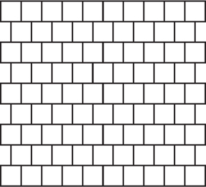
Figure 1 How to cover with squares so that no four overlap.

Here is another basic idea that leads to a useful definition of dimension, proposed by LEBESGUE [VI.72]. Suppose you want to cover an open interval of real numbers (that is, an interval that does not contain its endpoints) with shorter open intervals. Then you will be forced to make the shorter ones overlap, but you can do it in such a way that no point is contained in more than two of your intervals: just start each new interval close to the end of the previous one.

Now suppose that you want to cover an open square (that is, one that does not contain its boundary) with smaller open squares. Again you will be forced to make the smaller squares overlap, but this time the situation is slightly worse: some points will have to be contained in three squares. However, if you take squares arranged like bricks, as in figure 1, and expand them slightly, then you can do the covering in such a way that no four squares overlap. In general, it seems that to cover a typical d-dimensional set with small open sets, you need to have overlaps of d + 1 sets but you do not need to have overlaps greater than this.

The precise definition that this leads to is surprisingly general: it makes sense not just for subsets of ⁿ but even for an arbitrary TOPOLOGICAL SPACE [III.90]. We say that a set X is at most d dimensional if, however you cover X with a finite collection of open sets U1 , . . . , U_n, you can find a finite collection of open sets V1, . . . , V_m with the following properties:

(i) the sets V_i also cover the whole of X;

(ii) every V_i is a subset of at least one U_i;

(iii) no point is contained in more than d + 1 of the V_i.

If X is a metric space, then we can choose our U_i to have small diameter, thereby forcing the V_i to be small. So this definition is basically saying that it is possible to cover X with open sets with no d + 2 of them overlapping, and that these open sets can be as small as you like.

We then define the topological dimension of X to be the smallest d such that X is at most d dimensional. And again it can be shown that this definition assigns the “correct” dimension to the familiar shapes of elementary geometry.

A fourth intuitive idea leads to concepts known as homological and cohomological dimension. Associated with any suitable topological space X, such as a manifold, are sequences of groups known as HOMOLOGY AND COHOMOLOGY GROUPS [IV.6 §4]. Here we will discuss homology groups, but a very similar discussion is possible for cohomology. Roughly speaking, the nth homology group tells you how many interestingly different continuous maps there are from closed n-dimensional manifolds M to X. If X is a manifold of dimension less than n, then it can be shown that the nth homology group is trivial: in a sense, there is not enough room in X to define any map that is interestingly different from a constant map. On the other hand, the nth homology group of the n-sphere itself is , which says that one can classify the maps from the n-sphere to itself by means of an integer parameter.

It is therefore tempting to say that a space is at least n dimensional if there is room inside it for interesting maps from n-dimensional manifolds. This thought leads to a whole class of definitions. The homological dimension of a structure X is defined to be the largest n for which some substructure of X has a nontrivial n th homology group. (It is necessary to consider substructures, because homology groups can also be trivial when there is too much room: it then becomes easy to deform a continuous map and show that it is equivalent to a constant map.) However, homology is a very general concept and there are many different homology theories, so there are many different notions of homo-logical dimension. Some of these are geometric, but there are also homology theories for algebraic structures: for example, using suitable theories, one can define the homological dimension of algebraic structures such as RINGS [III.81 §1] or GROUPS [I.3 §2.1]. This is a very good example of geometrical ideas having an algebraic payoff.

Now let us turn to a fifth and final (for this article at least) intuitive idea about dimension, namely the way it affects how we measure size. If you want to convey how big a shape X is, then a good way of doing so is to give the length of X if X is one dimensional, the area if it is two dimensional, and the volume if it is three dimensional. Of course, this presupposes that you already know what the dimension is, but, as we shall see, there is a way of deciding which measure is the most appropriate without determining the dimension in advance. Then the tables are turned: we can actually define the dimension to be the number that corresponds to the best measure.

To do this, we use the fact that length, area, and volume scale in different ways when you expand a shape. If you take a curve and expand it by a factor of 2 (in all directions), then its length doubles. More generally, if you expand by a factor of C, then the length multiplies by C. However, if you take a two-dimensional shape and expand it by C, then its area multiplies by C². (Roughly speaking, this is because each little portion of the shape expands by C “in two directions” so you have to multiply the area by C twice.) And the volume of a three-dimensional shape multiplies by C³: for instance, the volume of a sphere of radius 3 is twenty-seven times the volume of a sphere of radius 1.

It may look as though we still have to decide in advance whether we will talk about length, area, or volume before we can even begin to think about how the measurement scales when we expand the shape. But this is not the case. For instance, if we expand a square by a factor of 2, then we obtain a new square that can be divided up into four congruent copies of the original square. So, without having decided in advance that we are talking about area, we can say that the size of the new square is four times that of the old square.

This observation has a remarkable consequence: there are sets to which it is natural to assign a dimension that is not an integer! Perhaps the simplest example is a famous set first defined by CANTOR [VI.54] and now known as the Cantor set. This set is produced as follows. You start with the closed interval [0,1], and call it X₀. Then you form a set X₁ by removing the middle third of X₀: that is, you remove all points between and but leave and themselves. So X₁ is the union of the closed intervals [0, ] and [ ,1]. Next, you remove the middle thirds of these two closed intervals to produce a set X₂, so X₂ is the union of the intervals [0, ], [, ], [, ], and [, 1].

In general, X_n is a union of closed intervals, and X_n+1 is what you get by removing the middle thirds of each of these intervals—so X_n+1 consists of twice as many intervals as X_n, but they are a third of the size. Once you have produced the sequence X₀, X₁, X₂, . . . , you define the Cantor set to be the intersection of all the X_i: that is, all the real numbers that remain, no matter how far you go with the process of removing middle thirds of intervals. It is not hard to show that these are precisely the numbers whose ternary expansions consist just of Os and 2s. (There are some numbers that have two different ternary expansions. For instance, can be written either as 0.1 or as 0.02222 . . . . In such cases we take the recurring expansion rather than the terminating one. So belongs to the Cantor set.) Indeed, when you remove middle thirds for the nth time, you are removing all numbers that have a 1 in the nth place after the “decimal” (in fact, ternary) point.

The Cantor set has many interesting properties. For example, it is UNCOUNTABLE [III.11], but it also has MEASURE [III.55] zero. Briefly, the first of these assertions follows from the fact that there is a different element of the Cantor set for every subset A of the natural numbers (just take the ternary number O.a₁a₂a₃ . . . , where a_i = 2 whenever i ∈ A and a_i = 0 otherwise), and there are uncountably many subsets of the natural numbers. To justify the second, note that the total length of the intervals making up X_n is ()ⁿ (since one removes a third of X_n–1 to produce X_n). Since the Cantor set is contained in every X_n, its measure must be smaller than ()ⁿ, whatever n is, which means that it must be zero. Thus, the Cantor set is very large in one respect and very small in another.

A further property of the Cantor set is that it is self-similar. The set X₁ consists of two intervals, and if you look at just one of these intervals as the middle thirds are repeatedly removed, then what you see is just like the construction of the whole Cantor set, but scaled down by a factor of 3. That is, the Cantor set consists of two copies of itself, each scaled down by a factor of 3. From this we deduce the following statement: if you expand the Cantor set by a factor of 3, then you can divide the expanded set up into two congruent copies of the original, so it is “twice as big.”

What consequence should this have for the dimension of the Cantor set? Well, if the dimension is d, then the expanded set ought to be 3^d times as big. Therefore, 3^d should equal 2. This means that d should be log 2 / log 3, which is roughly 0.63.

Once one knows this, the mystery of the Cantor set is lessened. As we shall see in a moment, a theory of fractional dimension can be developed with the useful property that a countable union of sets of dimension at most d has dimension at most d. Therefore, the fact that the Cantor set has dimension greater than 0 implies that it cannot be countable (since single points have dimension 0). On the other hand, because the dimension of the Cantor set is less than 1, it is much smaller than a one-dimensional set, so it is no surprise that its measure is zero. (This is a bit like saying that a surface has no volume, but now the two dimensions are 0.63 and 1 instead of 2 and 3.)

The most useful theory of fractional dimension is one developed by HAUSDORFF [VI.68]. One begins with a concept known as Hausdorff measure, which is a natural way of assessing the “d-dimensional volume” of a set, even if d is not an integer. Suppose you have a curve in ³ and you want to work out its length by considering how easy it is to cover it with spheres. A first idea might be to say that the length was the smallest you could make the sum of the diameters of the spheres. But this does not work: you might be lucky and find that a long curve was tightly wrapped up, in which case you could cover it with a single sphere of small diameter.

However, this would no longer be possible if your spheres were required to be small. Suppose, therefore, that we require all the diameters of the spheres to be at most δ. Let L(δ) be the smallest we can then get the sum of the diameters to be. The smaller δ is, the less flexibility we have, so the larger L (δ) will be. Therefore, L(δ) tends to a (possibly infinite) limit L as δ tends to 0, and we call L the length of the curve.

Now suppose that we have a smooth surface in ³ and want to deduce its area from information about covering it with spheres. This time, the area that you can cover with a very small sphere (so small that it meets only one portion of the surface and that portion is almost flat) will be roughly proportional to the square of the diameter of the sphere. But that is the only detail we need to change: let A(δ) be the smallest we can make the sum of the squares of the diameters of a set of spheres that cover the surface, if all those spheres have diameter at most δ. Then declare the area of the surface to be the limit of A(δ) as δ tends to 0. (Strictly speaking, we ought to multiply this limit by π/4, but then we get a definition that does not generalize easily.)

We have just given a way of defining length and area, for shapes in ³. The only difference between the two was that for length we considered the sum of the diameters of small spheres, while for area we considered the sum of the squares of the diameters of small spheres. In general, we define the d-dimensional Hausdorff measure in a similar way, but considering the sum of the dth powers of the diameters.

We can use the concept of Hausdorff measure to give a rigorous definition of fractional dimension. It is not hard to show that for any shape X there will be exactly one appropriate d, in the following sense: if c is less than d, then the c-dimensional Hausdorff measure of X is infinite, while if c is greater than d, then it is 0. (For instance, the c-dimensional Hausdorff measure of a smooth surface is 0 if c < 2 and infinite if c > 2.) This d is called the Hgusdorff dimension of the set X. Hausdorff dimension is very useful for analyzing fractal sets, which are discussed further in DYNAMICS [IV.14].

It is important to realize that the Hausdorff dimension of a set need not equal its topological dimension. For example, the Cantor set has topological dimension zero and Hausdorff dimension log 2/ log 3. A larger example is a very wiggly curve known as the Koch snowflake. Because it is a curve (and a single point is enough to cut it into two) it has topological dimension 1. However, because it is very wiggly, it has infinite length, and its Hausdorff dimension is in fact log 4/ log 3.