---

VII.03 Wavelets and Applications

Ingrid Daubechies

---

1 Introduction

One of the best ways to understand a function is to expand it in terms of a well-chosen set of “basic” functions, of which TRIGONOMETRIC FUNCTIONS [III.92] are perhaps the best-known example. Wavelets are families of functions that are very good building blocks for a number of purposes. They emerged in the 1980s from a synthesis of older ideas in mathematics, physics, electrical engineering, and computer science, and have since found applications in a wide range of fields. The following example, concerning image compression, illustrates several important properties of wavelets.

2 Compressing an Image

Directly storing an image on a computer uses a lot of memory. Since memory is a limited resource, it is highly desirable to find more efficient ways of storing images, or rather to find compressions of images. One of the main ways of doing this is to express the image as a function and write that function as a linear combination of basic functions of some kind. Typically, most of the coefficients in the expansion will be small, and if the basic functions are chosen in a good way it may well be that one can change all these small coefficients to zero without changing the original function in a way that is visually detectable.

Digital images are typically given by large collections of pixels (short for picture elements; see figure 1).

The boat image in figure 1 is made up of 256 × 384 pixels; each pixel has one of 256 possible gray values, ranging from pitch black to pure white. (Similar ideas apply to color images, but for this exposition, it is simpler to keep track of only one color.) Writing a number between 0 and 255 requires 8 digits in binary; the resulting 8-bit requirement to register the gray level for each of the 256 × 384 = 98 304 pixels thus gives a total memory requirement of 786 432 bits, for just this one image.

This memory requirement can be significantly reduced. In figure 2, two squares of 36×36 pixels are highlighted, in different areas of the image. As is clear from its blowup, square A has fewer distinctive characteristics than square B (a blowup of which is shown in figure 1), and should therefore be describable with fewer bits. Square B has more features, but it too contains (smaller) squares that consist of many similar pixels; again this can be used to describe this region with fewer than the 36 × 36 × 8 bits given by the naive estimate of assigning 8 bits to each pixel.

Figure 1 A digital image with successive blowups.

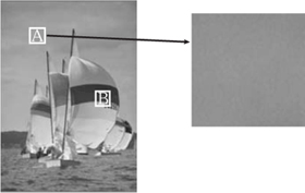
Figure 2 Blowup of a 36 × 36 square in the sky.

These arguments suggest that a change in the representation of the image can lead to reduced memory requirements: instead of a huge assembly of pixels, all equally small, the image should be viewed as a combination of regions of different size, each of which has more or less constant gray value; each such region can then be described by its size (or scale), by where it appears in the image, and by the 8-bit number that tells us its average gray value. Given any subregion of the image, it is easy to check whether it is already of this simple type by comparing it with its average gray value. For square A, taking the average makes virtually no difference, but for square B, the average gray value is not sufficient to characterize this portion of the image (see figure 3).

When square B is subdivided into yet smaller subsquares, some of them have a virtually constant gray level (e.g., in the top-left or bottom-left regions of square B); others, such as subsquares 2 and 3 (see figure 4), that are not of just one constant gray level may still have a simple gray level substructure that can be easily characterized with a few bits.

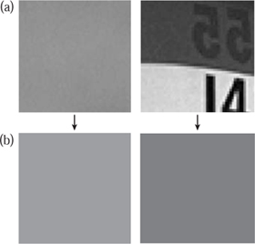
Figure 3 (a) Blowups of squares A (left) and B (right)with (b) the average gray value for each.

Figure 4 Subsquare 1 has constant gray level, while subsquares 2 and 3 do not, but they can be split horizontally (2) or vertically (3) into two regions with (almost) constant gray level. Subsquare 4 needs finer subdivision to be reduced to “simple” regions.

To use this decomposition for image compression, one should be able to implement it easily in an automated way. This could be done as follows:

• first, determine the average gray value for the whole image (assumed to be square, for simplicity);
• compare a square with this constant gray value with the original image; if it is close enough, then we are done (but it will have been a very boring image);
• if more features are needed than only the average gray value, subdivide the image into four equal-sized squares;
• for each of these subsquares, determine their average gray value, and compare with the subsquare itself;
• for those subsquares that are not sufficiently characterized by their average gray value, subdivide again into four further equal-sized subsquares (each now having an area one sixteenth of the original image);
• and so on.

In some of the subsquares it may be necessary to divide down to the pixel level (as in subsquare 4 in figure 4, for example), but in most cases subdivision can be stopped much earlier. Although this method is very easy to implement automatically, and leads to a description using many fewer bits for images such as the one shown, it is still somewhat wasteful. For instance, if the average gray level of the original image is 160, and we next determine the gray levels of each of the four quarter images as 224, 176, 112, and 128, then we have really computed one number too many: the average of the gray levels for the four equal-sized subimages is automatically the gray level of the whole image, so it is unnecessary to store all five numbers. In addition to the average gray value for a square, one just needs to store the extra information contained in the average gray values of its four quarters, given by the three numbers that describe

• how much darker (or lighter) the left half of the square is than the right,
• how much darker (or lighter) the top half of the square is than the bottom, and
• how much darker (or lighter) the diagonal from lower left to upper right is than the other diagonal.

Consider for example a square divided up into four subsquares with average values 224, 176, 112, and 128, as shown in figure 5. The average gray value for the whole square can easily be checked to be 160. Now let us do three further calculations. First, we work out the average gray values of the top half and the bottom half, which are 200 and 120, respectively, and calculate their difference, which is 80. Then we do the same for the left half and the right half, obtaining the difference 168 – 152 = 16. Finally, we divide the four squares up diagonally: the average over the bottom-left and top-right squares is 144, the average over the other two is 176, and the difference between these two is −32.

From these four numbers one can reconstruct the four original averages. For example, the average for the top-right subsquare is given by 160 + [80 − 16 + (−32)]/2 = 176.

Figure 5 The average gray values for four subsquares of a square.

It is thus this process, rather than simply averaging over smaller and smaller squares as described above, that needs to be repeated. We now turn to the question of making the whole decomposition procedure as efficient as possible.

A complete decomposition of a 256 × 256 square, from “top” (largest square) to “bottom” (the three types of “differences” for the 2 × 2 subsquares), involves the computation of many numbers (in fact exactly 256 × 256 before pruning), some of which are themselves combinations of many of the original pixel values. For instance, the grayscale average of the whole 256 × 256 square requires adding 256 × 256 = 65 536 numbers with values between 0 and 255 and then dividing the result by 65 536; another example, the difference between the averages of the left and right halves, requires adding the 256 × 128 = 32 768 grayscale numbers for the left half and then subtracting from this sum A the sum B of another 32 768 numbers. On the other hand, the sum of the pixel grayscale values over the whole square is simply A + B, a sum of two 33-bit numbers instead of 65 536 numbers of 8 bits each. This allows us to make a considerable saving in computational complexity if A and B are computed before the average over the whole square. A computationally optimal implementation of the ideas explained so far must therefore proceed along a different path from the one sketched above.

Indeed, a much better procedure is to start from the other end of the scale. Instead of starting with the whole image and repeatedly subdividing it, one begins at the pixel level and builds up. If the image has 2^J × 2^J pixels in total, then it can also be viewed as consisting of 2^J–1 × 2^J–1 “superpixels,” each of which is a small square of 2 × 2 pixels. For each 2 × 2 square, the average of the four gray values can be computed (this is the gray value of the superpixel), as well as the three types of differences indicated above. Moreover, these computations are all very simple.

The next step is to store the three difference values for each of the 2 × 2 squares and organize their averages, the gray values of the 2^J-1 × 2^J-1 superpixels, into a new square. This square can be divided, in turn, into 2^J-2 × 2^J-2 “super-superpixels,” each of which is a small square of 2 × 2 superpixels (and thus stands for 4 × 4 “standard” pixels), and so on. At the very end, after J levels of “zooming out,” there is only one super^J-pixel remaining; its gray value is the average over the whole image. The last three differences that were computed in this pixel-level-up process correspond exactly to the largest-scale differences that the top-down procedure would have computed first, at much greater computational expense.

Carrying out the procedure from the pixel level up, none of the individual averaging or differencing computations involves more than two numbers; the total number of these elementary computations, for the whole transform, is only 8(2^2J – 1)/3. For the 256×256 square discussed before, J = 8, so the total is 174 752, which is about the number of computations needed for just one level in the top-down procedure.

How can all this lead to compression? At each stage of the process, three species of difference numbers are accumulated, at different levels and corresponding to different positions. The total number of differences calculated is 3(1 + 2² + . . . + 2^2(J-1)) = 2^2J – 1. Together with the gray value of the whole square, this means we end up with exactly as many numbers as we had gray values for the original 2^J × 2^J pixels. However, many of these difference numbers will be very small (as argued before), and can just as well be dropped or put to zero, and if the image is reconstructed from the remainder there will be no perceptible loss of quality. Once we have set these very small differences to zero, a list that enumerates all the differences (in some prearranged order) can be made much shorter: whenever a long stretch of Z zeros is encountered, it can be replaced by the statement “insert Z zeros now,” which requires only a prearranged symbol (for “insert zeros now”), followed by the number of bits needed for Z, i.e., log₂ Z. This achieves, as desired, a significant compression of the data that need to be stored for large images. (In practice, however, image compression involves many more issues, to which we shall return briefly below.)

The very simple image decomposition described above is an elementary example of a wavelet decomposition. The data that are retained consist of

• a very coarse approximation, and
• additional layers giving detail at successively finer scales j, with j ranging from 0 (the coarsest level) to J – 1 (the first superpixel level).

Moreover, within each scale j the detail layer consists of many pieces, each of which has a definite localization (indicating to which of the super^j-pixels it pertains), and all the pieces have “size” 2^j. (That is, the size, in pixel widths, of the corresponding super^j-pixel is 2^j.) In particular, the building blocks are very small at fine scales and become gradually larger as the scale becomes coarser.

3 Wavelet Transforms of Functions

In the image-compression example we needed to look at three types of differences at each level (horizontal, vertical, and diagonal) because the example was a two-dimensional image. For a one-dimensional signal, one type of difference suffices. Given a function f from to , one can write a wavelet transform of f that is entirely analogous to the image example. For simplicity, let us look at a function f such that f(x) = 0 except when x belongs to the interval [0, 1].

Let us now consider successive approximations of f by step functions: that is, functions that change value in only finitely many places. More precisely, for each positive integer j, divide the interval [0, 1] up into 2^j equal intervals, denoting the interval from k2^-j to (k + 1)2^-j by I_j,k (so that k runs from 0 to 2^j- 1). Then define a function P_j(f) by setting its value on I_j,k to be the average value of f on that interval. This is illustrated in figure 6, which shows the step function P₃(f) for a function f whose graph is shown as well. As j increases, the width of the intervals I_j,k decreases, and P_j(f) gets closer to f. (In more precise mathematical terms, if p < ∞ and f belongs to the FUNCTION SPACE [III.29] L_p then P_J(f) converges to f in L_p.)

Each approximation P_j(f) of f can be computed easily from the approximation P_j+1 (f) at the next-finer scale: the average of the values that P_j+1 (f) takes on the two intervals I_j+1,2k and I_j+1,2k+1 gives the value that P_j(f) takes on I_{j, k}

Of course, some information about f is lost when we move from P_j+1(f) to P_j(f). On every interval I_j,k the difference between P_j+1(f) and P_j(f) is a step function, with constant levels on the I_j+1,l that takes on exactly opposite values on each pair (I_j+1,2k, I_j+1,2k+1). The difference P_j+1(f) – P_j(f) of the two approximation functions, over all of [0, 1], consists of a juxtaposition of such up-and-down (or down-and-up) step functions, and can therefore be written as a sum of translates of the same up-and-down function, with appropriate coefficients:

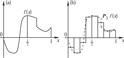
Figure 6 Graphs of (a) the function f and (b) its approximation P₃(f), which is constant on every interval between l/8 and (l + 1)/8, with l = 0,1, . . . ,7, and exactly equal to the average of f on each of these intervals.

where

Moreover, the “difference functions” U_j at the different levels are all scaled copies of a single function H, which takes the value 1 between 0 and and -1 between and 1; indeed, U_j(x) = H(2^jx). It follows that each difference P_j+1(f)(x) − P_j(f)(x) is a linear combination of the functions H(2^jx − k), with k ranging from 0 to 2^j − 1; adding many such differences, for successive j, shows that P_J(f)(x)−P₀(f)(x) is a linear combination of the collection of functions H(2^jx − k), with j ranging from 0 to J − 1 and k ranging from 0 to 2^j − 1. Picking larger and larger J makes P_J(f) closer and closer to f; one finds that f − P₀(f) (i.e., the difference between f and its average) can be viewed as a (possibly infinite) linear combination of the functions H(2^jx−k), now with j ranging over all the nonnegative integers.

This decomposition is very similar to what was done for images at the start of the article, but in one dimension instead of two and presented in a more abstract way. The basic ingredients are that f minus its average has been decomposed into a sum of layers at successively finer and finer scales, and that each extra layer of detail consists of a sum of simple “difference contributions” that all have width proportional to the scale. Moreover, this decomposition is realized by using translates and dilates of the single function H(x), often called the Haar wavelet, after Alfred Haar, who first defined it at the start of the twentieth century (though not in a wavelet context). The functions H(2^jx − k) constitute an orthogonal set of functions, meaning that the inner product ∫ H(2^jx − k)H(2^j′ x − k′) dx is zero except when j = j′ and k = k′; if we define H_j,k(x) = 2^j/2H(2^j x − k), then we also have that ∫ [H_j,k(x)]² dx = 1. A consequence of this is that the wavelet coefficients w_j,k(f) that appear when we write the “jth layer” P_j+1(f)(x) − P_j(f)(x) of the function f as a linear combination Σ_k w_j,k(f)H_j,k(x) are given by the formula W_j,k(f) = ∫ f(x)H_j,k (x) dx.

Haar wavelets are a good tool for exposition, but for most applications, including image compression, they are not the best choice. Basically, this is because replacing a function simply by its averages over intervals (in one dimension) or squares (in two dimensions) results in a very-low-quality approximation, as illustrated in figure 7(b).

As the scale of approximation is made finer and finer (i.e., as the j in P_j (f) increases), the difference between f and P_j(f) becomes smaller; with a piecewise-constant approximation, however, this requires corrections at almost every scale “to get it right” in the end. Unless the original happens to be made up of large areas where it is roughly constant, many small-scale Haar wavelets will be required even in stretches where the function just has a consistent, sustained slope, without “genuine” fine features.

The right framework to discuss these questions is that of approximation schemes. An approximation scheme can be defined by providing a family of “building blocks,” often with a natural order in which they are usually enumerated. A common way of measuring the quality of an approximation scheme is to define V_N to be the space of all linear combinations of the first N building blocks, and then to let A_N f be the closest function in V_N to f, where distance is measured by the L₂-norm (though other norms can also be used). Then one examines how the distance ||f − A_N f ||₂ = [∫ |f(x) − A_Nf (x)|² dx]^1/2 decays as N tends to infinity. An approximation scheme is said to be of order L for a class of functions if ||f − A_Nf ||₂ CN^-L for all functions f in , where C typically depends on f but must be independent of N. The order of an approximation scheme for smooth functions is closely linked to the performance of the approximation scheme on polynomials (because smooth functions can be replaced in estimations, at very little cost, by the polynomials given by their Taylor expansions). In particular, the types of approximation schemes considered here can have order L only if they perfectly reproduce polynomials of degree at most L – 1. In other words, there should exist some N₀ such that if p is any polynomial of degree at most L – 1 and N N_o, then A_N p = p.

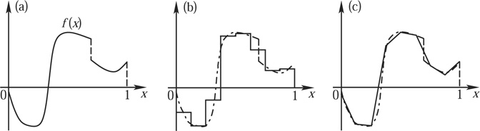
Figure 7 (a) The original function. (b), (c) Approximations of f by a function that equals a polynomial on each interval [k2^-3, (k + 1)2^-3). The best approximation of f by a piecewise-constant function is shown in (b); the best by a continuous piecewise-linear function is in (c).

In the Haar case, applied to functions f that differ from zero only between 0 and 1, the building blocks consist of the function that takes the value 1 on [0, 1] and 0 outside, together with the families {H_j,k; k = 0, . . . , 2^j – 1} for j = 0, 1, 2, . . . . We saw above that can be written as a linear combination of the first 1 + 2⁰ + 2¹ + . . . + 2^j-1 = 2^j building blocks H_0,0, H_1,0, H_1,1, H_2,0, . . . ,H_j-1,2^j-1-1. Because the Haar wavelets are orthogonal to each other, this is also the linear combination of these basis functions that is closest to f, so that Figure 7 shows (for j = 3) both and , which is the best approximation of f by a continuous, piecewise-linear function with breakpoints at k2^-j, k = 0, 1, . . . , 2^j-1. It turns out that if you are trying to approximate a function f using Haar wavelets, then the best decay you can obtain, even if f is smooth, is of the form or for N = 2^j. This means that approximation by Haar wavelets is a first-order approximation scheme. Approximation by continuous piecewise-linear functions is a second-order scheme: for smooth for N = 2^j. Note that the difference between the two schemes can also be seen from the maximal degree d of polynomials they “reproduce” perfectly: clearly both schemes can reproduce constants (d = 0); the piecewise-linear scheme can also reproduce linear functions (d = 1), whereas the Haar scheme cannot.

Take now any continuously differentiable function f defined on the interval [0, 1]. Typically ||f − ||₂ equals about C2^-j; for an approximation scheme of order 2, that same difference would be about C'2^-2j. In order to achieve the same accuracy as the piecewise-linear scheme would thus require only j/2 levels instead of j levels. For higher orders L, the gain would be even greater. If the projections P_j gave rise to a higher-order approximation scheme like this, then the difference P_j+1(f)(x) −P_j (f)(x) would be so small as not to matter, even for modest values of j, wherever the function f was reasonably smooth; for these values of j, the difference would be important only near points where the function was not as smooth, and so only in those places would a contribution be needed from “difference coefficients” at very fine scales.

This is a powerful motivation to develop a framework similar to that for Haar, but with fancier “generalized averages and differences” corresponding to successive P_j(f) associated with higher-order approximation schemes. This can be done, and was done in an exciting period in the 1980s to which we shall return briefly below. In these constructions, the generalized averages and differences are typically computed by combining more than two finer-scale entries each time, in appropriate linear combinations. The corresponding function decomposition represents functions as (possibly infinite) linear combinations of wavelets ψ_j,k derived from a wavelet ψ. As in the case of H, ψ_j,k(x) is defined to be 2^j/2ψ(2^j x − k). Thus, the functions ψ_j,k are again normalized translates and dilates of a single function; this is due to our using systematically the same averaging operator to go from scale j + 1 to scale j, and the same differencing operator to quantify the difference between levels j + 1 and j, regardless of the value of j. There is no absolutely compelling reason to use the same averaging and differencing operator for the transition between any two successive levels, and thus to have all the ψ_j,k generated by translating and dilating a single function. However, it is very convenient for implementing the transform, and it simplifies the mathematical analysis.

One can additionally require that, like the H_jk, the ψ_i,k constitute an orthonormal basis for the space L². The basis part means that every function can be written as a (possibly infinite) linear combination of the ψ_j,k; the orthonormality means that the ψ_j,k are orthogonal to each other, except if they are equal, in which case their inner product is 1.

As we have already mentioned, the projections P_j for the wavelet ψ will correspond to an approximation scheme of order L only if they can reproduce perfectly all polynomials of degree less than L. If the functions ψ_{j, k} are orthogonal, then ∫ ψ_j′,k(x)P_j(f)(x) dx = 0 whenever j′ > j. The ψ_j,k can thus be associated with an approximation scheme of order L only if ∫ ψ_{j, k}(x)p(x) dx = 0 for sufficiently large j and for all polynomials p of degree less than L. By scaling and translating, this reduces to the requirement ∫ x^lψ(x) dx = 0 for l = 0,1, . . . , L – 1. When this requirement is met, ψ is said to have L vanishing moments.

Figure 8 shows the graphs of some choices for ψ that give rise to orthonormal wavelet bases and that are used in various circumstances.

For the wavelets of the type ψ^[2n], and thus in particular for ψ^[4], ψ^[6], and ψ^[12] in figure 8, an algorithm similar to that for the Haar wavelet can be used to carry out the decomposition, except that instead of combining two numbers from P_j+1,k to obtain an average or a difference coefficient at level j, these wavelet decompositions require weighted combinations of four, six, or twelve finer-level numbers, respectively. (More generally, 2n finer-level numbers are used for ψ^[2n]

Because the Meyer and Battle-Lemarié wavelets ψ^[M] and ψ^[BL] are not concentrated on a finite interval, different algorithms are used for wavelet expansions with respect to these wavelets.

There are many useful orthonormal wavelet bases besides the examples given above. Which one to choose depends on the application one has in mind. For instance, if the function classes of interest in the application have smooth pieces, with abrupt transitions or spikes, then it is advantageous to pick a smooth ψ, corresponding to a high-order approximation scheme. This allows one to describe the smooth pieces efficiently with coarse-scale basis functions, and to leave the fine-scale wavelets to deal with the spikes and abrupt transitions. In that case, why not always use a wavelet basis with a very high approximation order? The reason is that most applications require numerical computation of wavelet transforms; the higher the order of the approximation scheme, the more spread out the wavelet, and the more terms have to be used in each generalized average/difference, which slows down numerical computation. In addition, the wider the wavelet, and hence the wider all the finer-scale wavelets derived from it, the more often a discontinuity or sharp transition will overlap with these wavelets. This tends to spread out the influence of such transitions over more fine-scale wavelet coefficients. Therefore, one must find a good balance between the approximation order and the width of the wavelet, and the best balance varies from problem to problem.

Figure 8 Six different choices of ψ for which the ψ_j,k(x) = 2^j/2ψ(2^jx – k), j,k ∈ , constitute an orthonormal basis for L² (). The Haar wavelet can be viewed as the first example of a family ψ^[2n], of which the wavelets for n = 2, 3, and 6 are also plotted here. Each ψ^[[2n] has n vanishing moments and is supported on (i.e., is equal to zero outside) an interval of width 2n – 1. The remaining two wavelets are not supported on an interval; however, the Fourier transform of the Meyer wavelet ψ^[M] is supported on [-8π/3, -2π/3] ∪ [2π/3, 8π/3]; all moments of ψ^[M] vanish. The Battle-Lemarié wavelet ψ^[BL] is twice differentiable, is piecewise polynomial of degree 3, and has exponential decay; it has four vanishing moments.

There are also wavelet bases in which the restriction of orthonormality is relaxed. In this case one typically uses two different “dual” wavelets ψ and , such that unless j = j′ and k = k′. The approximation order of the scheme that approximates functions f by linear combinations of the ψ_j,k is then governed by the number of vanishing moments of Such wavelet bases are called biorthogonal. They have the advantage that the basic wavelets ψ and can both be symmetric and concentrated on an interval, which is impossible for orthonormal wavelet bases other than the Haar wavelets.

The symmetry condition is important for image decomposition, where preference is usually given to two-dimensional wavelet bases derived from one-dimensional bases with a symmetric function ψ, a derivation to which we return below. When an image is compressed by deleting or rounding off wavelet coefficients, the difference between the original image I and its compressed version I^comp is a combination, with small coefficients, of these two-dimensional wavelets. It has been observed that the human visual system is more tolerant of such small deviations if they are symmetric; the use of symmetric wavelets thus allows for slightly larger errors, which translates to higher compression rates, before the deviations cross the threshold of perception or acceptability.

Another way of generalizing the notion of wavelet bases is to allow more than one starting wavelet. Such systems, known as multiwavelets, can be useful even in one dimension.

When wavelet bases are considered for functions defined on the interval [a, b] rather than the whole of R, the constructions are typically adapted, giving bases of interval wavelets in which specially crafted wavelets are used near the edges of the interval. It is sometimes useful to choose less regular ways of subdividing intervals than the systematic halving considered above: in this case, the constructions can be adapted to give irregularly spaced wavelet bases.

When the goal of a decomposition is compression of the information, as in the image example at the start, it is best to use a decomposition that is itself as efficient as possible. For other applications, such as pattern recognition, it is often better to use redundant families of wavelets, i.e., collections of wavelets that contain “too many” wavelets, in the sense that all functions in L²() could still be represented even if one dropped some of the wavelets from the collection. Continuous wavelet families and wavelet frames are the two main kinds of collections used for such redundant wavelet representations.

4 Wavelets and Function Properties

Wavelet expansions are useful for image compression because many regions of an image do not have features at very fine scales. Returning to the one-dimensional case, the same is true for a function that is reasonably smooth at most but not all points, like the function illustrated in figure 6(a). If we zoom in on such a function near a point x_o where it is smooth, then it will look almost linear, so we will be able to represent that part of the function efficiently if our wavelets are good at representing linear functions.

This is where wavelet bases other than Haar show their power: the wavelets ψ^[4], ψ^[6], ψ^[12], ψ^[M] and ψ^[BL] depicted in figure 8 all define approximation schemes of order 2 or higher, so that ∫ xψ_j,k(x) dx = 0 for all j, k. This is also seen in the numerical implementation schemes: the corresponding generalized differencing that computes the wavelet coefficients of f gives a zero result not only when the graph is flat, but also when it is a straight but sloped line, which is not true for the simple differencing used for the Haar basis. As a result, the number of coefficients needed for the wavelet expansion of smooth functions f to reach a preassigned accuracy is much smaller when one uses more sophisticated wavelets than the Haar wavelets.

For a function f that is twice differentiable except at a finite number of discontinuities, and with a basic wavelet that has, say, three vanishing moments, typically only very few wavelets at fine scales will be needed to write a very-high-precision approximation to f. Moreover, those will be needed only near the discontinuity points. This feature is characteristic for all wavelet expansions, whether they are with respect to an orthonormal basis, a basis that is nonorthogonal, or even a redundant family.

Figure 9 illustrates this for one type of redundant expansion, which uses the so-called Mexican hat wavelets, which are given by this wavelet gets its name from the shape of its graph, which looks like the cross section of a Mexican hat (see the figure).

The smoother a function f is (i.e., the more times it is differentiable), the faster its wavelet coefficients will decay as j increases, provided the wavelet ψ has sufficiently many vanishing moments. The converse statement is also true: one can read off how smooth the function is at x₀ from how the wavelet coefficients w_j,k (f) decay, as j increases. Here one restricts attention to the “relevant” pairs (j, k). In other words, one considers only the pairs where ψ_j,k is localized near x₀. (In more precise terms, this converse statement can be reformulated as an exact characterization of the so-called Lipschitz spaces C^α, for all noninteger a that are strictly less than the number of vanishing moments of ψ.)

Figure 9 A function with a single discontinuity (top) is approximated by finite linear combinations of Mexican hat wavelets ψ^[MH]_j.l; the graph of ψ^[MH] is at the bottom of the figure. Adding finer scales leads to increased precision. Left: successive approximations for j = 1, 3, 5, and 7. Right: total contributions from the wavelets at the scales needed to bridge from one j to the next. (In this example, j increases in steps of ) The finer the scale, the more the extra detail is concentrated near the discontinuity point.

Wavelet coefficients can be used to characterize many other useful properties of functions, both global and local. Because of this, wavelets are good bases not just for L²-spaces or the Lipschitz spaces, but also for many other function spaces, such as, for instance, the L^p-spaces with 1 < p < ∞, the SOBOLEV SPACES [III.29§2.4], and a wide range of Besov spaces. The versatility of wavelets is partly due to their connection with powerful techniques developed in harmonic analysis throughout the twentieth century.

We have already seen in some detail that wavelet bases are associated with approximation schemes of different orders. So far we have considered approximation schemes in which the A_Nf are always linear combinations of the same N building blocks, regardless of the function f. This is called linear approximation, because the collection of all functions of the form A_Nf is contained in the linear span V_N of the first N basis functions. Some of the function spaces mentioned above can be characterized by specifying the decay of ||f − A_Nf ||₂ as N increases, where A_N is defined in terms of an appropriate wavelet basis.

However, when it is compression that we are interested in, we are really carrying out a different kind of approximation. Given a function f, and a desired accuracy, we want to approximate f to within that accuracy by a linear combination of as few basis functions as possible, but we are not trying to choose those functions from the first few levels. In other words, we are no longer interested in the ordering of the basis functions and we do not prefer one label (j, k) over another.

If we want to formalize this, we can define an approximation A_Nf to be the closest linear combination to f that is made up of at most N basis functions. By analogy with linear approximation, we can then define the set _N as the set of all possible linear combinations of _N basis functions. However, the sets _N are no longer linear spaces: two arbitrary elements _N are typically combinations of two different collections of N basis functions, so that their sum has no reason to belong to VN (though it will belong to _2N). For this reason, A_Nf is called a nonlinear approximation of f.

One can go further and define classes of functions by imposing conditions on the decay of ||f − A_Nf ||, as N increases, with respect to some function space norm || · ||. This can of course be done starting from any basis; wavelet bases distinguish themselves from many other bases (such as the trigonometric functions) in that the resulting function spaces turn out to be standard function spaces, such as the Besov spaces, for example. We have referred several times to functions that are smooth in many places but have possible discontinuities in isolated points, and argued that they can be approximated well by linear combinations of a fairly small number of wavelets. Such functions are special cases of elements of particular Besov spaces, and their good approximation properties by sparse wavelet expansions can be viewed as a consequence of the characterization of these Besov spaces by nonlinear approximation schemes using wavelets.¹

5 Wavelets in More than One Dimension

There are many ways to extend the one-dimensional constructions to higher dimensions. An easy way to construct a multidimensional wavelet basis is to combine several one-dimensional wavelet bases. The image decomposition at the start is an example of such a combination: it combines two one-dimensional Haar decompositions. We saw earlier that a 2 × 2 superpixel could be decomposed as follows. First, think of it as arranged in two rows of two numbers, representing the gray levels of the corresponding pixels. Next, for each row replace its two numbers by their average and their difference, obtaining a new 2 × 2 array. Finally, do the same process to the columns of the new array. This produces four numbers, the result of, respectively,

• averaging both horizontally and vertically,
• averaging horizontally and differencing vertically,
• differencing horizontally and averaging vertically, and
• differencing both horizontally and vertically.

The first is the average gray level for the superpixel, which is needed as the input for the next round of the decomposition at the next scale up. The other three correspond to the three types of “differences” already encountered earlier. If we start with a rectangular image that consists of 2^K rows, each containing 2^J pixels, then we end up with 2^K-1 × 2^J-1 numbers of each of the four types. Each collection is naturally arranged in a rectangle of half the size of the original (in both directions); it is customary in the image-processing literature to put the rectangle with gray values for the superpixels in the top left; the other three rectangles each group together all the differences (or wavelet coefficients) of the other three kinds. (See the level 1 decomposition in figure 10.) The rectangle that results from horizontal differencing and vertical averaging typically has large coefficients at places where the original image has vertical edges (such as the boat masts in the example above); likewise, the horizontal averaging/vertical differencing rectangle has large coefficients for horizontal edges in the original (such as the stripes in the sails); the horizontal differencing/vertical differencing rectangle selects for diagonal features. The three different types of “difference terms” indicate that we have here three basic wavelets (instead of just one in the one-dimensional case).

In order to go to the next round, one scale up, the scenario is repeated on the rectangle that contains the superpixel gray values (the results of averaging both horizontally and vertically); the other three rectangles are left unchanged. figure 10 shows the result of this process for the original boat image, though the wavelet basis used here is not the Haar basis, but a symmetric biorthogonal wavelet basis that has been adopted in the JPEG 2000 image compression standard. The result is a decomposition of the original image into its component wavelets. The fact that so much of this is gray indicates that a lot of this information can be discarded without affecting the image quality.

figure 11 illustrates that the number of vanishing moments is important not just when the wavelet basis is used for characterizing properties of functions, but also when it comes to image analysis. It shows an image that has been decomposed in two different ways: once with Haar wavelets, the other with the JPEG 2000 standard biorthogonal wavelet basis. In both cases, all but the largest 5% of the wavelet coefficients have been set to zero, and we are looking at the corresponding reconstructions of the images, neither of which is perfect. However, the wavelet used in the JPEG 2000 standard has four vanishing moments, and therefore gives a much better approximation in smoothly varying parts of the image than the Haar basis. Moreover, the reconstruction obtained from the Haar expansion is “blockier” and less attractive.

6 Truth in Advertising: Closer to True Image Compression

Image compression has been discussed several times in this article, and it is indeed a context in which wavelets are used. However, in practice there is much more to image compression than the simple idea of dropping all but the largest wavelet coefficients, taking the resulting truncated list of coefficients, and replacing each of the many long stretches of zeros by its runlength. In this short section we shall give a glimpse of the large gap between the mathematical theory of wavelets as discussed above and the real-life practice of engineers who want to compress images.

First of all, compression applications set a “bit budget,” and all the information to be stored has to fit within the bit budget; statistical estimates and information-theoretic arguments about the class of images under consideration are used to allocate different numbers of bits to different types of coefficients. This bit allocation is much more gradual and subtle than just retaining or dropping coefficients. Even so, many coefficients will get no bits assigned to them, meaning that they are indeed dropped altogether.

Figure 10 Wavelet decomposition of the boat image, together with a grayscale rendition of the wavelet coefficients. The decompositions are shown after one level of averaging and differencing, as well as after two and three levels. In the rectangles corresponding to wavelet coefficients (i.e., not averaged in both directions), where numbers can be negative, the convention is to use gray scale 128 for zero, and darker/lighter gray scales for positive and negative values. The wavelet rectangles are mostly at gray scale 128, indicating that most of the wavelet coefficients are negligibly small.

Figure 11 Top: original image, with blowup. Bottom: approximations obtained by expanding the image into a wavelet basis, and discarding the 95% smallest wavelet coefficients. Left: Haar wavelet transform. Right: wavelet transform using the so-called 9-7 biorthogonal wavelet basis.

Because some coefficients are dropped, care has to be taken that each of the remaining coefficients is given its correct address, i.e., its (j,k_l, k₂) label, which is essential for “decompressing” the stored information in order to reconstruct the image (or rather, an approximation to it). If you do not have a good strategy for doing this, then you can easily find that the computational resources needed to encode information about the addresses cancel out a large portion of the gain made by the nonlinear wavelet approximation. Every practical wavelet-based image-compression scheme uses some sort of clever approach to deal with this problem. One implementation exploits the observation that at locations in the image where wavelet coefficients of some species are negligibly small at some scale j, the wavelet coefficients of the same species at finer scales are often very small as well. (Check it out on the boat image decomposition given above.) At each such location, this method sets a whole tree of finer-scale coefficients (four for scale j + 1, sixteen for scale j + 2, etc.) automatically to zero; for those locations where this assumption is not borne out by the wavelet coefficients that are obtained from the actual decomposition of the image at hand, extra bits must then be spent to store the information that a correction has to be made to the assumption. In practice, the bits gained by the “zero-trees” far outweigh the bits needed for these occasional corrections.

Depending on the application, many other factors can play a role. For instance, if the compression algorithm has to be implemented in an instrument on a satellite where it can only draw on very limited power supplies, then it is also important for the computations involved in the transform itself to be as economical as possible.

Readers who want to know more about (important!) considerations of this kind can find them discussed in the engineering literature. Readers who are content to stay at the lofty mathematical level are of course welcome to do so, but are hereby warned that there is more to image compression via wavelet transforms than has been sketched in the previous sections.

7 Brief Overview of Several Influenceson the Development of Wavelets

Most of what is now called “wavelet theory” was developed in the 1980s and early 1990s. It built on existing work and insights from many fields, including harmonic analysis (mathematics), computer vision and computer graphics (computer science), signal analysis and signal compression (electrical engineering), coherent states (theoretical physics), and seismology (geophysics). These different strands did not come together all at once but were brought together gradually, often as the result of serendipitous circumstances and involving many different agents.

In harmonic analysis, the roots of wavelet theory go back to work by LITTLEWOOD [VI.79] and Paley in the 1930s. An important general principle in Fourier analysis is that the smoothness of a function is reflected in its FOURIER TRANSFORM [III.27]: the smoother the function, the faster the decay of its transform. Little-wood and Paley addressed the question of characterizing local smoothness. Consider, for example, a periodic function with period 1 that has just one discontinuity in the interval [0, 1) (which is then repeated at all integer translates of that point), and is smooth elsewhere. Is the smoothness reflected in the Fourier transform?

If the question is understood in the obvious way, then the answer is no: a discontinuity causes the Fourier coefficients to decay slowly, however smooth the rest of the function is. Indeed, the best possible decay is of the form . If there were no discontinuity, the decay would be at least as good as C_k [1 +|n|]^−k when f is k-times differentiable.

However, there is a more subtle connection between local smoothness and Fourier coefficients. Let f be a periodic function, and let us write its nth Fourier coefficient as a_ne^iθn, where a_n is the absolute value of and e^iθn is its phase. When examining the decay of the Fourier coefficients, we look just at a_n and forget all about the phases, which means that we cannot detect any phenomenon unless it is unaffected by arbitrary changes to the phases. If f has a discontinuity, then we can clearly move it about by changing the phases. It turns out that these phases play an important role in determining not just where the singularities are, but even their severity: if the singularity at x_o is not just a discontinuity but a divergence of the type |f(x)| ˜ |x − x_o|^−ß, then one can change the value of ß just by changing the phases and without altering the absolute values |a_n|. Thus, changing phases in Fourier series is a dangerous thing to do: it can greatly change the properties of the function in question.

Littlewood and Paley showed that some changes of the phases of Fourier coefficients are more innocuous. In particular, if you choose a phase change for the first Fourier coefficient, another one for both the next two coefficients, another for the next four, another for the next eight, and so on, so that the phase changes are constant on “blocks” of Fourier coefficients that keep doubling in length, then local smoothness (or absence of smoothness) properties of f are preserved. Similar statements hold for the Fourier transform of functions on (as opposed to Fourier series of periodic functions). This was the first result of a whole branch of harmonic analysis in which scaling was exploited systematically to deal with detailed local analysis, and in which very powerful theorems were proved that, with hindsight, seem ready-made to establish a host of powerful properties for wavelet decompositions. The simplest way to see the connection between Littlewood-Paley theory and wavelet decompositions is to consider the Shannon wavelet ψ^[sh], which is defined by ^[sh] (ξ) = 1 when π |ξ| < 2π, and ^[sh](ξ) = 0 otherwise. Here, ^[sh] denotes the Fourier transform of the wavelet ψ^[sh]. The corresponding functions ψ^[sh]_j,k(x) = 2^j/2ψ^[Sh](2^jx − k) constitute an orthonormal basis for L² (), and for each f and each j the collection of inner products tells us how (ξ) restricts to the set 2^j−1 π⁻¹|ξ| < 2^j. In other words, it gives us the jth Littlewood-Paley block of f.

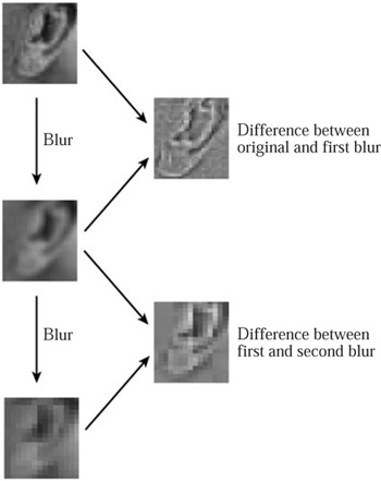
Figure 12 Differences between successiveblurs give detail at different scales.

Scaling also plays an important role in computer vision, where one of the basic ways to “understand” an image (going back to at least the early 1970s) is to blur it more and more, erasing more detail each time, so as to obtain approximations that are graded in “coarseness” (see figure 12). Details at different scales can then be found by considering the differences between successive coarsenings. The relationship with wavelet transforms is obvious!

An important class of signals of interest to electrical engineers is that of bandlimited signals, which are functions f, usually of one variable only, for which the Fourier transform vanishes outside some interval. In other words, the frequencies that make up f come from some “limited band.” If the interval is [-Ω, Ω], then f is said to have bandlimit Ω. Such functions are completely characterized by their values, often called samples, at integer multiples of π/Ω. Most manipulations on the signal f are carried out not directly but by operations on this sequence of samples. For instance, we might want to restrict f to its “lower-frequency half.” To do this, we would define a function g by the condition that (ξ) = (ξ) if |ξ| Ω/2 and is 0 otherwise. Equivalently, we could say that (ξ) = (ξ)(ξ), where (ξ) = 1 if |ξ| Ω/2 and 0 otherwise. The next step is to let L_n be L(nπ/Ω), and we find that g(kπ/Ω) = Σ_n∈L_n f ((k − n)π/Ω). To put this more neatly, if we write a_n and _n for f(nπ/Ω) and g(nπ/Ω), respectively, then _k = Σ_n∈L_na_k−n. On the other hand, g clearly has bandlimit Ω/2, so to characterize g it suffices to know only the sequence of samples at integer multiples of 2π/Ω. In other words, we just need to know the numbers b_k = _2k. The transition from f to g is therefore given by b_k= Σ_n∈L_na_2k−n. In the appropriate electrical engineering vocabulary, we have gone from a critically sampled sequence for f (i.e., its sampling rate corresponded exactly to its bandlimit) to a critically sampled sequence for g by filtering (multiplying by some function, or convolving the sequence (f(nπ/Ω))_n∈ with a sequence of filter coefficients) and downsampling (retaining only one sample in two, because these are the only samples necessary to characterize the more narrowly bandlimited g). The upper-frequency half h of f can be obtained by the inverse Fourier transform of the restriction of (ξ) to |ξ| > Ω/2. Like g, the function h is also completely characterized by its values at multiples of 2π/Ω, and h can also be obtained from f by filtering and downsampling. This split of f into its lower and upper frequency halves, or subbands, is thus given by formulas that are the exact equivalent of the generalized averaging and differencing encountered in the implementation of wavelet transforms for orthonormal wavelet bases supported on an interval. Subband filtering followed by critical downsampling had been developed in the electrical engineering literature before wavelets came along, but were typically not concatenated in several stages.

A concept of central importance in quantum physics is that of a UNITARY REPRESENTATION [IV.15 §1.4] of a LIE GROUP [III.48 §1] on some HILBERT SPACE [III.37]. In other words, given a Lie group G and a Hilbert space H, one interprets the elements g of G as unitary transformations of H. The elements of H are called states, and for certain Lie groups, if υ is some fixed state, then the family of vectors {gυ g ∈ G} is called a family of coherent states. Coherent states go back to work by Schrödinger in the 1920s. Their name dates back to the 1950s, when they were used in quantum optics: the word “coherent referred to the coherence of the light they were describing. These families turned out to be of interest in a much wider range of settings in quantum physics, and the name stuck, even outside the original setting of optics. In many applications it helps not to use the whole family of coherent states but only those coherent states that correspond to a certain kind of discrete subset of G. Wavelets turn out to be just such a subfamily of coherent states: one starts with a single, basic wavelet, and the transformations that convert it (by dilation and translation) into the remaining wavelets form a discrete semigroup of such transformations.

Despite the fact that wavelets synthesized ideas from all these fields, their discovery originated in another area altogether. In the late 1970s, the geophysicist J. Morlet was working for an oil company. Dissatisfied with the existing techniques for extracting special types of signals from seismograms, he came up with an ad hoc transform that combined translations and scalings: nowadays, it would be called a redundant wavelet transform. Other transforms in seismology with which Morlet was familiar involve comparing the seismic traces with special functions of the form W_m,n(t) = w(t − nτ) cos(mωt), where w is a smooth function that gently rises from 0 to 1 and then gently decays to 0 again, all within a finite interval. Several different examples of functions w, proposed by several different scientists, are used in practice: because the functions W_m,n look like small waves (they oscillate, but have a nice beginning and end because of w) they are typically called “wavelets of X,” named after proposer X for that particular w. The reference functions in Morlet’s new ad hoc family, which he used to compare pieces of seismic traces, were different in that they were produced from a function w by scaling instead of multiplying them by increasingly oscillating trigonometric functions. Because of this, they always had the same shape, and Morlet called them “wavelets of constant shape” (see figure 13) in order to distinguish them from the wavelets of X (or Y, or Z, etc.).

Morlet taught himself to work with this new transform and found it numerically useful, but had difficulty explaining his intuition to others because he had no underlying theory. A former classmate pointed him in the direction of A. Grossmann, a theoretical physicist, who made the connection with coherent states and, together with Morlet and other collaborators, started to develop a theory for the transform in the early 1980s. Outside the field of geophysics it was no longer necessary to use the phrase “of constant shape,” so this was quickly dropped, which annoyed geophysicists when, some years later, more mature forms of wavelet theory impinged on their field again.

Figure 13 Top: an example of a window function w that is used in practice by geophysicists, with just below it two examples of w (t− nτ) e^imt i.e., two “traditional” geophysics wavelets. Bottom: a wavelet as used by Morlet, with two translates and dilates just below it—these have constant shape, unlike the “traditional” ones.

A few years later, in 1985, standing in line for a photocopy machine at his university, harmonic analysis expert Y. Meyer heard about this work and realized it presented an interestingly different take on the scaling techniques with which he and other harmonic analysts had long been familiar At the time, no wavelet bases were known in which the initial function ψ combined the properties of smoothness and good decay. Indeed, there seemed to be a subliminal expectation in papers on wavelet expansions that no such orthonormal wavelet bases could exist. Meyer set out to prove this, and to everyone's surprise and delight he failed in the best possible way—by finding a counterexample, the first smooth wavelet basis! Except that it later turned out not to have been the very first: a few years before, a different harmonic analyst, O. Stromberg, had constructed a different example, but this had not attracted attention at the time.

Meyer’s proof was ingenious, and worked because of some seemingly miraculous cancellations, which is always unsatisfactory from the point of view of mathematical understanding. Similar miracles played a role in independent constructions by P. G. Lemarié (now Lemarié-Rieusset) and G. Battle of orthonormal wavelet bases that were piecewise polynomial. (They came to the same result from completely different points of departure—harmonic analysis for Lemarié and quantum field theory for Battle.)

A few months later, S. Mallat, then a Ph.D. candidate in computer vision in the United States, learned about these wavelet bases. He was on vacation, chatting on the beach with a former classmate who was one of Meyer’s graduate students. After returning to his Ph.D. work, Mallat kept thinking about a possible connection with the reigning paradigm in computer vision. On learning that Meyer was coming to the United States in the fall of 1986 to give a named lecture series, he went to see him and explain his insight. In a few days of feverish enthusiasm, they hammered out multiresolution analysis, a different approach to Meyer’s construction inspired by the computer vision framework. In this new setting, all the miracles fell into place as inevitable consequences of simple, entirely natural construction rules, embodying the principle of successively finer approximations. Multiresolution analysis has remained the basic principle behind the construction of many wavelet bases and redundant families

None of the smooth wavelet bases constructed up to that point was supported inside an interval, so the algorithms to implement the transform (which were using the subband filtering framework without their creators knowing that it had been named and developed in electrical engineering) required, in principle, infinite filters that were impossible to implement. In practice, this meant that the infinite filters from the mathematical theory had to be truncated; it was not clear how to construct a multiresolution analysis that would lead to finite filters. Truncation of the infinite filters seemed to me a blemish on the whole beautiful edifice, and I was unhappy with this state of affairs. I had learned about wavelets from Grossmann and about multiresolution analysis from explanations scribbled by Meyer on a napkin after dinner during a conference. In early 1987 I decided to insist on finite filters for the implementation. I wondered whether a whole multiresolution analysis (and its corresponding orthonormal basis of wavelets) could be reconstructed from appropriate but finite filters. I managed to carry out this program, and as a result found the first construction of an orthonormal wavelet basis for which ψ is smooth and supported on an interval.

Soon after this, the connection with the electrical engineering approaches was discovered. Especially easy algorithms were inspired by the needs of computer graphics applications. More exciting constructions and generalizations followed: biorthogonal wavelet bases, wavelet packets, multiwavelets, irregularly spaced wavelets, sophisticated multidimensional wavelet bases not derived from one-dimensional constructions, and so on.

It was a heady, exciting period. The development of the theory benefited from all the different influences and in its turn enriched the different fields with which wavelets are related. As the theory has matured, wavelets have become an accepted addition to the mathematical toolbox used by mathematicians, scientists, and engineers alike. They have also inspired the development of other tools that are better adapted to tasks for which wavelets are not optimal.

Further Reading

Aboufadel, E., and S. Schlicker. 1999. Discovering Wavelets. New York: Wiley Interscience.

Blatter, C. 1999. Wavelets: A Primer. Wellesley, MA: AK Peters.

Cipra, B. A. 1993. Wavelet applications come to the fore. SIAM News 26(7):10-11, 15.

Frazier, M. W. 1999. An Introduction to Wavelets through Linear Algebra. New York: Springer.

Hubbard, B. B. 1995. The World According to Wavelets: The Story of a Mathematical Technique in the Making. Wellesley, MA: AK Peters.

Meyer, Y., and R. Ryan. 1993. Wavelets: Algorithms and Applications. Philadelphia, PA: Society for Industrial and Applied Mathematics (SIAM).

Mulcahy, C. 1996. Plotting & scheming with wavelets. Mathematics Magazine 69(5):323-43.

1. More types of wavelet families, as well as many generalizations, can be found on the Internet at www.wavelet.org.