
IV.26 High-Dimensional Geometry and Its Probabilistic Analogues
Keith Ball
1 Introduction
If you have ever watched a child blowing soap bubbles, then you cannot have failed to notice that the bubbles are, at least as far as the human eye can tell, perfectly spherical. From a mathematical perspective, the reason for this is simple. The surface tension in the soap solution causes each bubble to make its area as small as possible, subject to the constraint that it encloses a fixed amount of air (and cannot compress the air too much). The sphere is the surface of smallest area that encloses a given volume.
As a mathematical principle, this seems to have been recognized by the ancient Greeks, although fully rigorous demonstrations did not appear until the end of the nineteenth century. This and similar statements are known as “isoperimetric principles.”1

Figure 1 A soap film has minimum area.
The two-dimensional form of the problem asks: what is the shortest curve that encloses a given area? The answer, as we might expect by analogy with the three-dimensional case, is a circle. Thus, by minimizing the length of the curve we force it to have a great deal of symmetry: the curve should be equally curved everywhere along its length. In three or more dimensions, many different kinds of CURVATURE [III.78] are used in different contexts. One, known as mean curvature, is the appropriate one for area-minimization problems.
The sphere has the same mean curvature at every point, but then it is pretty clear from its symmetry that the sphere would have the same curvature at every point whatever measure of curvature we used. More illustrative examples are provided by the soap films (much more varied than simple bubbles) that are a popular feature of recreational mathematics lecturesfigure 1 shows such a soap film stretched across a wire frame. The film adopts the shape that minimizes its area, subject to the constraint that it is bounded by the wire frame. One can show that the minimal surface (the exact mathematical solution to the minimization problem) has constant mean curvature: its mean curvature is the same at every point.
Isoperimetric principles turn up all over mathematics: in the study of partial differential equations, the calculus of variations, harmonic analysis, computational algorithms, probability theory, and almost every branch of geometry. The aim of the first part of this article is to describe a branch of mathematics, high-dimensional geometry, whose starting point is the fundamental isoperimetric principle: that the sphere is the surface of least area that encloses a given volume. The most remarkable feature of high-dimensional geometry is its intimate connection to the theory of probability: geometric objects in high-dimensional space exhibit many of the characteristic properties of random distributions. The aim of the second part of this article is to outline the links between the geometry and probability.
2 High-Dimensional Spaces
So far we have discussed only two- and three-dimensional geometry. Higher-dimensional spaces seem to be impossible for humans to visualize but it is easy to provide a mathematical description of them by extending the usual description of three-dimensional space in terms of Cartesian coordinates. In three dimensions, a point (x,y,z) is given by three coordinates; in n-dimensional space, the points are n-tuples (x1, x2, . . ., xn). As in two and three dimensions, the points are related to one another in that we can add two of them together to produce a third, by simply adding corresponding coordinates:
(2, 3, . . ., 7) + (1, 5, . . ., 2) = (3, 8, . . ., 9).
By relating points to one another, addition gives the space some structure or “shape.” The space is not just a jumble of unrelated points.
To describe the shape of the space completely, we also need to specify the distance between any two points. In two dimensions, the distance of a point (x,y) from the origin is ![]() by the Pythagorean theorem (and the fact that the axes are perpendicular). Similarly, the distance between two points (u, v) and (x,y) is
by the Pythagorean theorem (and the fact that the axes are perpendicular). Similarly, the distance between two points (u, v) and (x,y) is
![]()
In n dimensions we define the distance between points (u1, u2, . . ., un) and (x1, x2, . . ., xn) to be
![]()
Volume is defined in n-dimensional space roughly as follows. We start by defining a cube in n dimensions. The two- and three-dimensional cases, the square and the usual three-dimensional cube, are very familiar The set of all points in the xy-plane whose coordinates are between 0 and 1 is a square of side 1 unit (as shown in figure 2), and, similarly, the set of all points (x,y,z) for which x, y, and z are all between 0 and 1 is a unit cube. In n-dimensional space the analogous cube consists of those points whose coordinates are all between 0 and 1. We stipulate that the unit cube has volume 1. Now, if we double the size of a plane figure, its area increases by a factor of 4. If we double a three-dimensional body, its volume increases by a factor of 8. In n-dimensional space, the volume scales as the nth power of size: so a cube of side t has volume tn. To find the volume of a more general set we try to approximate it by covering it with little cubes whose total volume is as small as possible. The volume of the set is calculated as a limit of these approximate volumes.

Whatever the dimension, a special geometric role is played by the unit sphere: that is, the surface consisting of all points that are a distance of 1 unit from a fixed point, the center. As one might expect, the corresponding solid sphere, or unit ball, consisting of all points enclosed by the unit sphere, also plays a special role. There is a simple relationship between the (n-dimensional) volume of the unit ball and the (n - 1)-dimensional “area” of the sphere. If we let νn denote the volume of the unit ball in n dimensions, then the surface area is nνn. One way to see this is to imagine enlarging the unit ball by a factor slightly greater than 1, say 1 + ε. This is pictured in figure 3. The enlarged ball has volume (1 + ε)nνn and so the volume of the shell between the two spheres is ((1 + ε)n - 1) νn. Since the shell has thickness ε, this volume is approximately the surface area multiplied by ε. So the surface area is approximately
![]()
By taking the limit as ε approaches 0 we obtain the surface area exactly:
![]()
One can check that this limit is nνn either by expanding the power (1 + ε)n or by observing that the expression is the formula for a derivative.
So far we have discussed bodies in n-dimensional space without being too precise about what kind of sets we are considering. Many of the statements in this article hold true for quite general sets. But a special role is played in high-dimensional geometry by convex sets (a set is convex if it contains the entire line segment joining any two of its points). Balls and cubes are both examples of convex sets. The next section describes a fundamental principle which holds for very general sets but which is intrinsically linked to the notion of convexity.

3 The Brunn–Minkowski Inequality
The two-dimensional isoperimetric principle was essentially proved in 1841 by Steiner, although there was a technical gap in the argument which was filled later. The general (n-dimensional) case was completed by the end of the nineteenth century. A couple of decades later a different approach to the principle, with far-reaching consequences, was found by HERMANN MINKOWSKI [VI.64]—an approach which was inspired by an idea of Hermann Brunn.
Minkowski considered the following way to add together two sets in n-dimensional space. If C and D are sets, then the sum C + D consists of all points which can be obtained by adding a point of C to a point of D. figure 4 shows an example in which C is an equilateral triangle and D is a square centered at the origin. We place a copy of the square at each point of the triangle (some of these are illustrated) and the set C + D consists of all points that are included in all these squares. The outline of C + D is shown dashed.
The Brunn–Minkowski inequality relates the volume of the sum of two sets to the volumes of the sets themselves. It states that (as long as the two sets C and D are not empty)
![]()
The inequality looks a bit technical, if only because the volumes appearing in the inequality are raised to the power 1/n. However, this fact is crucial. If each of C and D is a unit cube (with their edges aligned the same way), then the sum C + D is a cube of side 2: a cube twice as large. Each of C and D has volume 1 while the volume of C + D is 2n. So, in this case, vol(C + D)1/n = 2 and each of vol(C)1/n and vol(D)1/n is equal to 1: the inequality (1) holds with equality. Similarly, whenever C and D are copies of one another, the Brunn–Minkowski inequality holds with equality. If we omitted the exponents 1/n, the statement would still be true; in the case of two cubes, it is certainly true that 2n ≥ 1 + 1. But the statement would be extremely weak: it would give us almost no useful information.

The importance of the Brunn–Minkowski inequality stems from the fact that it is the most fundamental principle relating volume to the operation of addition, which is the operation that gives space its structure. At the start of this section it was explained that Minkowski’s formulation of Brunn’s idea provided a new approach to the isoperimetric principle. Let us see why.
Let C be a COMPACT SET [III.9] in ![]() n whose volume is equal to that of the unit ball B. We want to show that the surface area of C is at least n vol(B) since this is the surface area of the ball. We consider what happens to C if we add a small ball to it. An example (a right-angled triangle) is shown in figure 5: the dashed curve outlines the enlarged set we obtain by adding to C a copy of the ball B scaled by a small factor ε. This looks rather like figure 3 above but here we do not expand the original set, we add a ball. Just as before, the difference between C + εB and C is a shell around C of width ε, so we can express the surface area as a limit as ε approaches 0:
n whose volume is equal to that of the unit ball B. We want to show that the surface area of C is at least n vol(B) since this is the surface area of the ball. We consider what happens to C if we add a small ball to it. An example (a right-angled triangle) is shown in figure 5: the dashed curve outlines the enlarged set we obtain by adding to C a copy of the ball B scaled by a small factor ε. This looks rather like figure 3 above but here we do not expand the original set, we add a ball. Just as before, the difference between C + εB and C is a shell around C of width ε, so we can express the surface area as a limit as ε approaches 0:
![]()
Now the Brunn–Minkowski inequality tells us that
vol(C + εB)1/n ≥ vol(C)1/n + vol(εB)1/n.

The right-hand side of this inequality is
vol(C)1/n + ε vol(B)1/n = (1 + ε) vol(B)1/n
because vol(εB) = εn vol(B) and vol(C) = vol(B). So the surface area is at least

Again as in section 2, this limit is n vol(B) and we conclude that the surface of C has at least this area.
Over the years, many different proofs of the Brunn–Minkowski inequality have been found, and most of the methods have other important applications. To finish this section we shall describe a modified version of the Brunn-Minkowski inequality that is often easier to use than (1). If we replace the set C + D by a scaled copy half as large, ![]() (C + D), then its volume is scaled by 1/2n and the nth root of this volume is scaled by
(C + D), then its volume is scaled by 1/2n and the nth root of this volume is scaled by ![]() . Therefore, the inequality can be rewritten
. Therefore, the inequality can be rewritten
![]()
Because of the simple inequality ![]() x +
x + ![]() y ≥
y ≥ ![]() for positive numbers, the right-hand side of this inequality is at least
for positive numbers, the right-hand side of this inequality is at least ![]() . It follows that
. It follows that
![]()
and hence that
![]()
We shall elucidate a striking consequence of this inequality in the next section.
The Brunn–Minkowski inequality holds true for very general sets in n-dimensional space, but for convex sets it is the beginning of a surprising theory that was initiated by Minkowski and developed in a remarkable way by Aleksandrov, Fenchel, and Blaschke, among others: the theory of so-called mixed volumes. In the 1970s Khovanskii and Teissier (using a discovery of D. Bernstein) found an astonishing connection between the theory of mixed volumes and the Hodge index theorem in algebraic geometry.

Figure 6 Expanding half a ball.
4 Deviation in Geometry
Isoperimetric principles state that if a set is reasonably large, then it has a large surface or boundary. The Brunn–Minkowski inequality (and especially the argument we used to deduce the isoperimetric principle) expands upon this statement by showing that if we start with a reasonably large set and extend it (by adding a small ball), then the volume of the new set is quite a lot bigger than that of the original. During the 1930s Paul Lévy realized that in certain situations, this fact can have very striking consequences. To get an idea of how this works suppose that we have a compact set C inside the unit ball, whose volume is half that of the ball; for example, C might be the set pictured in figure 6.
Now extend the set C by including all points of the ball that are within distance ε of C, much as we did when deducing the isoperimetric inequality (the dashed curve in figure 6 shows the boundary of the extended set). Let D denote the remainder of the ball (also illustrated). Then if c is a point in C and d is a point in D, we are guaranteed that c and d are separated by a distance of at least ε. A simple two-dimensional argument, pictured in figure 7, shows that in this case the midpoint ![]() (c + d) cannot be too near the surface of the ball. In fact, its distance from the center is no more than 1 -
(c + d) cannot be too near the surface of the ball. In fact, its distance from the center is no more than 1 - ![]() ε2. So the set
ε2. So the set ![]() (C + D) lies inside the ball of radius 1 -
(C + D) lies inside the ball of radius 1 - ![]() ε2, whose volume is (1 –
ε2, whose volume is (1 – ![]() ε2)n times the volume of the ball νn. The crucial point is that if the exponent n is large and ε is not too small, the factor (1 –
ε2)n times the volume of the ball νn. The crucial point is that if the exponent n is large and ε is not too small, the factor (1 – ![]() ε2)n is extremely small: in a space of high dimension, a ball of slightly smaller radius has very much smaller volume. In order to make use of this we apply inequality (2), which states that the volume of
ε2)n is extremely small: in a space of high dimension, a ball of slightly smaller radius has very much smaller volume. In order to make use of this we apply inequality (2), which states that the volume of ![]() (C + D) is at leaxst
(C + D) is at leaxst ![]() . Therefore,
. Therefore,

Figure 7 A two-dimensional argument.
![]()
It is convenient to replace the factor (1 - ![]() ε2)2n by a (pretty accurate) approximation e-nε2/4 which is slightly easier to understand. We can then conclude that the volume vol(D) of the residual set D satisfies the inequality
ε2)2n by a (pretty accurate) approximation e-nε2/4 which is slightly easier to understand. We can then conclude that the volume vol(D) of the residual set D satisfies the inequality
![]()
If the dimension n is large, then the exponential factor e-nε2/4 is very small, as long as ε is a bit bigger than 1/![]() . What this means is that only a small fraction of the ball lies in the residual set D. All but a small fraction of the ball lies close to C, even though some points in the ball may lie much farther from C. Thus, if we start with a set (any set) that occupies half the ball and extend it a little bit, we swallow up almost the entire ball. With a little more sophistication, the same argument can be used to show that the surface of the ball, the sphere, has exactly the same property. If a set C occupies half the sphere, then almost all of the sphere is close to that set.
. What this means is that only a small fraction of the ball lies in the residual set D. All but a small fraction of the ball lies close to C, even though some points in the ball may lie much farther from C. Thus, if we start with a set (any set) that occupies half the ball and extend it a little bit, we swallow up almost the entire ball. With a little more sophistication, the same argument can be used to show that the surface of the ball, the sphere, has exactly the same property. If a set C occupies half the sphere, then almost all of the sphere is close to that set.
This counterintuitive effect turns out to be characteristic of high-dimensional geometry. During the 1980s a startling probabilistic picture of high-dimensional space was developed from Lévy’s basic idea. This picture will be sketched in the next section.
One can see why the high-dimensional effect has a probabilistic aspect if one thinks about it in a slightly different way. To begin with, let us ask ourselves a basic question: what does it mean to choose a random number between 0 and 1? It could mean many things but if we want to specify one particular meaning, then our job is to decide what the chance is that the random number will fall into each possible range a ≤ × ≤ b: what is the chance that it lies between 0.12 and 0.47, for example? For most people, the obvious answer is 0.35, the difference between 0.47 and 0.12. The probability that our random number lands in the interval a ≤ × ≤ b will just be b - a, the length of that interval. This way of choosing a random number is called uniform. Equal-sized parts of the range between 0 and 1 are equally likely to be selected.
Just as we can use length to describe what is meant by a random number, we can use the volume measure in n-dimensional space to say what it means to select a random point of the n-dimensional ball. We have to decide what the chance is that our random point falls into each subregion of the ball. The most natural choice is to say that it is equal to the volume of that subregion divided by the volume of the entire ball, that is, the proportion of the ball occupied by the subregion. With this choice of random point, it is possible to reformulate the high-dimensional effect in the following way. If we choose a subset C of the ball which has a ![]() chance of being hit by our random point, then the chance that our random point lies more than ε away from C is no more than 2e-nε2/4
chance of being hit by our random point, then the chance that our random point lies more than ε away from C is no more than 2e-nε2/4
To finish this section it will be useful to rephrase the geometric deviation principle as a statement about functions rather than sets. We know that if C is a set occupying half the sphere, then almost the entire sphere is within a small distance of C. Now suppose that f is a function defined on the sphere: f assigns a real number to each point of the sphere. Assume that f cannot change too rapidly as you move around the sphere: for example, that the values f(x) and f(y) at two points x and y cannot differ by more than the distance between x and y. Let M be the median value of f, meaning that f is at most M on half the sphere and at least M on the other half. Then it follows from the deviation principle that f must be almost equal to M on all but a small fraction of the sphere. The reason is that almost all of the sphere is close to the half where f is below M; so f cannot be much more than M except on a small set. On the other hand, almost all of the sphere is close to the half where f is at least M; so f cannot be much less than M except on a small set.
Thus, the geometric deviation principle says that if a function on the sphere does not vary too fast, then it must be almost constant on almost the entire sphere (even though there may be some points where it is very far from this constant value).
5 High-Dimensional Geometry
It was mentioned at the end of section 3 that convex sets have a special significance in Minkowski’s theory relating volume to the additive structure of space. They also occur naturally in a large number of applications: in linear programming and partial differential equations, for example. Although convexity is a fairly restrictive condition for a body to satisfy, it is not hard to convince oneself that convex sets exhibit considerable variety and that this variety seems to increase with the dimension. The simplest convex sets after the balls are cubes. If the dimension is large, the surface of a cube looks very unlike the sphere. Let us consider, not a unit cube, but a cube of side 2 whose center is the origin. The corners of the cube are points like (1, 1, . . ., 1) or (1, -1, -1, . . ., 1), whose coordinates are all equal to 1 or -1, while the center of each face is a point like (1, 0, 0, . . ., 0) which has just one coordinate equal to 1 or -1. The corners are at a distance ![]() from the center of the cube, while the centers of the faces are at distance 1 from the origin. Thus, the largest sphere that can be fitted inside the cube has radius 1, while the smallest sphere that encloses the cube has radius
from the center of the cube, while the centers of the faces are at distance 1 from the origin. Thus, the largest sphere that can be fitted inside the cube has radius 1, while the smallest sphere that encloses the cube has radius ![]() (this is illustrated in figure 8).
(this is illustrated in figure 8).
When the dimension n is large, this ratio of ![]() is also large. As one might expect, this gap between the ball and the cube is able to accommodate a wide variety of different convex shapes. Nevertheless, the probabilistic view of high-dimensional geometry has led to an understanding that, for many purposes, this enormous variety is an illusion: that in certain well-defined senses, all convex bodies behave like balls.
is also large. As one might expect, this gap between the ball and the cube is able to accommodate a wide variety of different convex shapes. Nevertheless, the probabilistic view of high-dimensional geometry has led to an understanding that, for many purposes, this enormous variety is an illusion: that in certain well-defined senses, all convex bodies behave like balls.
Probably the first discovery that pointed strongly in this direction was made by Dvoretzky in the late 1960s. Dvoretzky’s theorem says that every high-dimensional convex body has slices that are almost spherical. More precisely, if you specify a dimension (say ten) and a degree of accuracy, then for any sufficiently large dimension n, every n-dimensional convex body has a ten-dimensional slice that is indistinguishable from a ten-dimensional sphere, up to the specified accuracy.
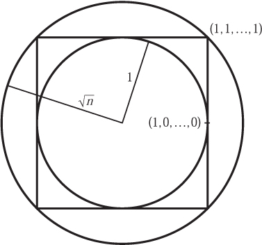
Figure 8 A ball in a box in a ball.

Figure 9 The directional radius.
The proof of Dvoretzky’s theorem that is conceptually simplest depends upon the deviation principle described in the last section and was found by Milman a few years after Dvoretzky’s theorem appeared. The idea is roughly this. Consider a convex body K in n dimensions that contains the unit ball. For each point θ on the sphere, imagine the line segment starting at the origin, passing through the sphere at θ, and extending out to the surface of K (see figure 9). Think of the length of this line as the “radius” of K in the direction of θ and call it r(θ). This “directional radius” is a function on the sphere. Our aim is to find (say) a 10-dimensional slice of the sphere on which r(θ) is almost constant. In such a slice, the body K looks like a ball, since its radius hardly varies.
The fact that K is convex means that the function r cannot change too rapidly as we move around the sphere: if two directions are close together, then the radius of K must be about the same in these two directions. Now we apply the geometric deviation principle to conclude that the radius of N is roughly the same on almost the entire sphere: the radius is close to its average (or median) value for all but a small fraction of the possible directions. That means that we have plenty of room in which to go looking for a slice on which the radius is almost constant—we just have to choose a slice that avoids the small bad regions. It can be shown that this happens if we choose the slice at random from among all possible slices. The fact that most of the sphere consists of good regions means that a random slice has a good chance of falling into a good region.
Dvoretzky’s theorem can be recast as a statement about the behavior of the entire body K, rather than just its sections, by using the Minkowski sums defined in the previous section. The statement is that if K is a convex body in n dimensions, then there is a family of m rotations K1, K2, . . ., Km of K whose Minkowski sum K1 + · · · + Km is approximately a ball, where the number m is significantly smaller than the dimension n. Recently, Milman and Schechtman realized that the smallest number m that would work could be described almost exactly, in terms of relatively simple properties of the body K, despite the apparently enormous complexity of the choice of rotations available.
For some n-dimensional convex sets, it is possible to create a ball with many fewer than n rotations. In the late 1970s Kašin discovered that if K is the cube, then just two rotations K1 and K2 are enough to produce something approximating a ball, even though the cube itself is extremely far from spherical. In two dimensions it is not hard to work out which rotations are best: if we choose K1 to be a square and K2 to be its rotation through 45°, then K1 + K2 is a regular octagon which is as close to a circle as we can get with just two squares. In higher dimensions it is extremely hard to describe which rotations to use. At present the only known method is to use randomly chosen rotations, even though the cube is as concrete and explicit an object as one ever meets in mathematics.
The strongest principle discovered to date showing that most bodies behave like balls is what is usually called the reverse Brunn–Minkowski inequality. This result was proved by Milman, building on ideas of his own and of Pisier and Bourgain. The Brunn–Minkowski inequality was stated earlier for sums of bodies. The reverse one has a number of different versions; the simplest is in terms of intersections. To begin with, if K is a body and B is a ball of the same volume, then the intersection of these two sets, the region that they have in common, is clearly of smaller volume. This obvious fact can be stated in a complicated way that looks like the Brunn–Minkowski inequality:
![]()
If K is extremely long and thin, then whenever we intersect it with a ball of the same volume, we capture only a tiny part of K. So there is no possibility of reversing inequality (4) as it stands: no possibility of estimating the volume of K ∩ B from below. But if we are allowed to stretch the ball before intersecting it with K, the situation changes completely. A stretched ball in n-dimensional space is called an ellipsoid (in two dimensions it is just an ellipse). The reverse Brunn–Minkowski inequality states that for every convex body K, there is an ellipsoid ![]() of the same volume for which
of the same volume for which
![]()
where α is a fixed positive number.
There is a widespread (but not quite universal) belief that an apparently much stronger principle is true: that if we are allowed to enlarge the ellipsoid by a factor of (say) 10, then we can ensure that it includes half the volume of K. In other words, for every convex body, there is an ellipsoid of roughly the same size that contains half of K. Such a statement flies in the face of our intuition about the huge variety of shapes in high dimensions, but there are some good reasons to believe it.
Since the Brunn–Minkowski inequality has a reverse form, it is natural to ask whether the isoperimetric inequality also does. The isoperimetric inequality guarantees that sets cannot have a surface that is too small. Is there a sense in which bodies cannot have too large a surface area? The answer is yes, and indeed a rather precise statement can be made. Just as in the case of the Brunn–Minkowski inequality, we have to take into account the possibility that our body could be long and thin and so have small volume but very large surface. So we have to start by applying a linear transformation that stretches the body in certain directions (but does not bend the shape). For example, if we start with a triangle, we first transform it into an equilateral triangle and then measure its surface and its volume. Once we have transformed our body as best we can, it turns out that we can specify precisely which convex body has the largest surface for a given volume. In two dimensions it is the triangle, in three it is the tetrahedron, and in n dimensions it is the natural analogue of these: the n-dimensional convex set (called a simplex) which has n + 1 corners. The fact that this set has the largest surface was proved by the present author using an inequality from harmonic analysis discovered by Brascamp and Lieb; the fact that the simplex is the only convex set with maximal surface (in the sense described) was proved by Barthe.
In addition to geometric deviation principles, two other methods have played a central role in the modern development of high-dimensional geometry; these methods grew out of two branches of probability theory. One is the study of sums of random points in NORMED SPACES [III.62] and how big they are, which provides important geometrical information about the spaces themselves. The other, the theory of Gaussian processes, depends upon a detailed understanding of how to cover sets in high-dimensional space efficiently with small balls. This issue may sound abstruse but it addresses a fundamental problem: how to measure (or estimate) the complexity of a geometric object. If we know that our object can be covered by one ball of radius 1, ten balls of radius ![]() , fifty-seven balls of radius
, fifty-seven balls of radius ![]() , and so on, then we have a good idea of how complicated the object can be.
, and so on, then we have a good idea of how complicated the object can be.
The modern view of high-dimensional space has revealed that it is at once much more complicated than was previously thought and at the same time in other ways much simpler. The first of these is well illustrated by the solution of a problem posed by Borsuk in the 1930s. A set is said to have diameter at most d if no two points in the set are further than d from each other. In connection with his work in topology, Borsuk asked whether every set of diameter 1 in n-dimensional space could be broken into n + 1 pieces of smaller diameter. In two and three dimensions this is always possible, and as late as the 1960s it was expected that the answer should be yes in all dimensions. However, a few years ago, Kahn and Kalai showed that in n dimensions it might require something like e![]() pieces, enormously more than n + 1.
pieces, enormously more than n + 1.
On the other hand, the simplicity of high-dimensional space is reflected in a fact discovered by Johnson and Lindenstrauss: if we pick a configuration of n points (in whatever dimension we like), we can find an almost perfect copy of the configuration sitting in a space of dimension much smaller than n: roughly the logarithm of n. In the last few years this fact has found applications in the design of computer algorithms, since many computational problems can be phrased geometrically and become much simpler if the dimension involved is small.
6 Deviation in Probability
If you toss a fair coin repeatedly, you expect that heads will occur on roughly half the tosses, and tails on roughly half. Moreover, as the number of tosses increases, you expect the proportion of heads to get closer and closer to ![]() . The number
. The number ![]() is called the expected number of heads per toss. The number of heads yielded by a given toss is either 1 or 0, with equal probability, so the expected number of heads is the average of these, namely
is called the expected number of heads per toss. The number of heads yielded by a given toss is either 1 or 0, with equal probability, so the expected number of heads is the average of these, namely ![]() .
.
The crucial unspoken assumption that we make about the tosses of the coin is that they are independent: that the outcomes of different tosses do not influence one another. (Independence and other basic probabilistic concepts are discussed in PROBABILITY DISTRIBUTIONS [III.71].) The coin-tossing principle, or its generalization to other random experiments, is called the strong law of large numbers. The average of a large number of independent repetitions of a random quantity will be close to the expected value of the quantity.
The strong law of large numbers for coin tosses is fairly simple to demonstrate. The general form, which applies to much more complicated random quantities, is considerably more difficult. It was first established by KOLMOGOROV [VI.88] in the early part of the twentieth century.
The fact that averages accumulate near the expected value is certainly useful to know, but for most purposes in statistics and probability theory it is vital to have more detailed information. If we focus our attention near the expected value, we may ask how the average is distributed around this number. For example, if the expected value is ![]() , as for coin tossing, we might ask, what is the chance that the average is as large as 0.55 or as small as 0.42? We want to know how likely it is that our average number of heads will deviate from the expected value by a given amount.
, as for coin tossing, we might ask, what is the chance that the average is as large as 0.55 or as small as 0.42? We want to know how likely it is that our average number of heads will deviate from the expected value by a given amount.
The bar chart in figure 10 shows the probabilities of obtaining each of the possible numbers of heads, with twenty tosses of a coin. The height of each bar shows the chance that the corresponding number of heads will occur. As we would expect from the strong law of large numbers, the taller bars are concentrated near the middle. Superimposed upon the chart is a curve that plainly approximates the probabilities quite well. This is the famous “bell-shaped” or “normal” curve. It is a shifted and rescaled copy of the so-called standard normal curve, whose equation is

Figure 10 Twenty tosses of a fair coin.
![]()
The fact that the curve approximates coin-tossing probabilities is an example of the most important principle in probability theory: the central limit theorem. This states that whenever we add up a large number of small independent random quantities, the result has a distribution that is approximated by a normal curve.
The equation of the normal curve (5) can be used to show that if we toss a coin n times, then the chance that the proportion of heads deviates from ![]() by more than ε is at most e-2nε2. This closely resembles the geometric deviation estimate (3) from section 4. This resemblance is not coincidental, although we are still far from a full understanding of when and how it applies.
by more than ε is at most e-2nε2. This closely resembles the geometric deviation estimate (3) from section 4. This resemblance is not coincidental, although we are still far from a full understanding of when and how it applies.
The simplest way to see why a version of the central limit theorem might apply to geometry is to replace the toss of a coin by a different random experiment. Suppose that we repeatedly select a random number between -1 and 1, and that the selection is uniform in the sense described in section 4. Let the first n selections be the numbers x1, x2, . . ., xn. Instead of thinking of them as independent random choices, we can consider the point (x1, . . ., xn) as a randomly chosen point inside the cube that consists of all points whose coordinates lie between -1 and 1. The expression (1/![]() )
) ![]() measures the distance of the random point from a certain (n - 1)-dimensional “plane,” which consists of all points whose coordinates add up to zero (the two-dimensional case is shown in figure 11). So the chance that (1/
measures the distance of the random point from a certain (n - 1)-dimensional “plane,” which consists of all points whose coordinates add up to zero (the two-dimensional case is shown in figure 11). So the chance that (1/![]() )
) ![]() deviates from its expected value, 0, by more than ε is the same as the chance that a random point of the cube lies a distance of more than ε from the plane. This chance is proportional to the volume of the set of points that are more than ε from the plane: the set shown shaded in figure 11. When we discussed the geometric deviation principle, we estimated the volume of the set of points which were more than ε away from a set C which occupied half the ball. The present situation is really the same, because each part of the shaded set consists of those points that are more than ε away from whichever half of the cube lies on the other side of the plane.
deviates from its expected value, 0, by more than ε is the same as the chance that a random point of the cube lies a distance of more than ε from the plane. This chance is proportional to the volume of the set of points that are more than ε from the plane: the set shown shaded in figure 11. When we discussed the geometric deviation principle, we estimated the volume of the set of points which were more than ε away from a set C which occupied half the ball. The present situation is really the same, because each part of the shaded set consists of those points that are more than ε away from whichever half of the cube lies on the other side of the plane.

Figure 11 A random point of the cube.
Arguments akin to the central limit theorem show that if we cut the cube in half with a plane, then the set of points which lie more than a distance ε from one of the halves has volume no more thane e-ε2. This statement is different from, and apparently much weaker than, the one we obtained for the ball (3) because the factor of n is missing from the exponent. The estimate implies that if you take any plane through the center of the cube, then most points in the cube will be at a distance of less than 2 from it. If the plane is parallel to one of the faces of the cube, this statement certainly is weak, because all of the cube is within distance 1 of the plane. The statement becomes significant when we consider planes like the one in figure 11. Some points of the cube are at a distance of ![]() from this “diagonal” plane, but still, the overwhelming majority of the cube is very much closer. Thus, the estimates for the cube and the ball contain essentially the same information; what is different is that the cube is bigger than the ball by a factor of about
from this “diagonal” plane, but still, the overwhelming majority of the cube is very much closer. Thus, the estimates for the cube and the ball contain essentially the same information; what is different is that the cube is bigger than the ball by a factor of about ![]() .
.
In the case of the ball we were able to prove a deviation estimate for any set occupying half the ball, not just the special sets that are cut off by planes. Towards the end of the 1980s Pisier found an elegant argument that showed that the general case works for the cube as well as for the ball. Among other things, the argument uses a principle which goes back to the early days of large-deviation theory in the work of Donsker and Varadhan.
The theory of large deviations in probability is now highly developed. In principle, more or less precise estimates are known for the probability that a sum of independent random variables deviates from its expectation by a given amount, in terms of the original distribution of the variables. In practice, the estimates involve quantities that may be difficult to compute, but there are sophisticated methods for doing this. The theory has numerous applications within probability and statistics, computer science, and statistical physics.
One of the most subtle and powerful discoveries of this theory is Talagrand’s deviation inequality for product spaces, discovered in the mid 1990s. Talagrand himself has used this to solve several famous problems in combinatorial probability and to obtain striking estimates for certain mathematical models in particle physics. The full inequality of Talagrand is somewhat technical and is difficult to describe geometrically. However, the discovery had a precursor which fits perfectly into the geometric picture and which captures at least one of the most important ideas.2 We look again at random points in the cube but this time the random point is not chosen uniformly from within the cube. As before, we choose the coordinates x1, x2, . . ., xn of our random point independently of one another, but we do not insist that each coordinate is chosen uniformly from the range between -1 and 1. For example, it might be that xl can take only the values 1, 0, or -1, each with probability ![]() that x2 can take only the values 1 or -1 each with probability
that x2 can take only the values 1 or -1 each with probability ![]() , and perhaps that x3 is chosen uniformly from the entire range between -1 and 1. What matters is that the choice of each coordinate has no effect on the choice of any others.
, and perhaps that x3 is chosen uniformly from the entire range between -1 and 1. What matters is that the choice of each coordinate has no effect on the choice of any others.
Any sequence of rules that dictates how we choose each coordinate determines a way of choosing a random point in the cube. This in turn gives us a way of measuring a kind of volume for subsets of the cube: the “volume” of a set A is the chance that our random point is selected from A. This way to measure volume might be very different from the usual one; among other things, an individual point might have nonzero volume.
Now suppose that C is a convex subset of the cube and that its “volume” is ![]() in the sense that our random point will be selected from C with probability
in the sense that our random point will be selected from C with probability ![]() . Talagrand’s inequality says that the chance that our random point will lie a distance of more than ε from C is less than 2e-ε2/16. This statement looks like the deviation estimate for the cube except that it refers only to convex sets C. But the crucial new information that makes the estimate and its later versions important is that we are allowed to choose our random point in so many different ways.
. Talagrand’s inequality says that the chance that our random point will lie a distance of more than ε from C is less than 2e-ε2/16. This statement looks like the deviation estimate for the cube except that it refers only to convex sets C. But the crucial new information that makes the estimate and its later versions important is that we are allowed to choose our random point in so many different ways.
This section has described deviation estimates in probability theory that have a geometric flavor. For the cube, we are able to show that if C is any set occupying half the cube, then almost the entire cube is close to C. It would be extremely useful to know the same thing for convex sets more general than the cube. There are some other highly symmetric sets for which we do know it, but the most general possible statement of this type seems to be beyond our current methods. One potential application, which comes from theoretical computer science, is to the analysis of random algorithms for volume calculation. The problem may sound specialized, but it arises in LINEAR PROGRAMMING [III.84] (which alone is sufficient reason to justify the expenditure of enormous effort) and in the numerical estimation of integrals. In principle, one can calculate the volume of a set by laying over it a very fine grid, and counting how many grid points fall into the set. In practice, if the dimension is large, the number of grid points will be so astronomically huge that no computer has a chance of performing the count.
The problem of calculating the volume of a set is essentially the same as the problem of choosing a point at random within the set, roughly as we saw in section 4. So the aim is to select a random point without identifying a huge number of possible points to select from. At present, the most effective way of generating a random point in a convex set is to carry out a random walk within the set. We perform a sequence of small steps whose directions are chosen randomly and then select the point that we have reached after a fairly large number of steps, in the hope that this point has roughly the correct chance of falling into each part of the set. For the method to be effective, it is essential that the random walk quickly visits points all over the set: that it does not get stuck for a long time in, say, half of the set. In order to guarantee this rapid mixing, as it is called, we need an isoperimetric principle or deviation principle. We need to know that each half of our set has a large boundary, so that there is a good chance that our random walk will cross the boundary quickly and land in the other half of our set.
In a series of papers published over the last ten years, Applegate, Bubley, Dyer, Frieze, Jerrum, Kannan, Lovasz, Montenegro, Simonovits, Vempala, and others have found very efficient random walks for sampling from a convex set. A geometric deviation principle of the kind alluded to above would make it possible to estimate the efficiency of these random walks almost perfectly.
7 Conclusion
The study of high-dimensional systems has become increasingly important in the last few decades. Practical problems in computing frequently lead to high-dimensional questions, many of which can be posed geometrically, while many models in particle physics are automatically high-dimensional because it is necessary to consider a huge number of particles in order to mimic large-scale phenomena in the real world. The literature in both these fields is vast but some general remarks can be made. The intuition that we gain from low-dimensional geometry leads us wildly astray if we try to apply it in many dimensions. It has become clear that naturally occurring high-dimensional systems exhibit characteristics that we expect to arise in probability theory, even if the original system does not have an explicitly random element. In many cases these random characteristics are manifested as an isoperimetric or deviation principle, that is, a statement to the effect that large sets have large boundaries. In the classical theory of probability, independence assumptions can often be used to demonstrate deviation principles quite simply. For the very much more complicated systems that are studied today it is usually useful to have a geometric picture to accompany the probabilistic one. That way one can understand probabilistic deviation principles as analogues of the isoperimetric principle discovered by the ancient Greeks. This article has described the relationship between geometry and probability in just a few special cases. A very much more detailed picture is almost certainly waiting to be found. At present it seems to be just out of reach.
Further Reading
Ball, K. M. 1997. An elementary introduction to modern convex geometry. In Flavors of Geometry, edited by Silvio Levy. Cambridge: Cambridge University Press.
Bollobás, B. 1997. Volume estimates and rapid mixing. In Flavors of Geometry, edited by Silvio Levy. Cambridge: Cambridge University Press.
Chavel, I. 2001. Isoperimetric Inequalities. Cambridge: Cambridge University Press.
Dembo, A., and O. Zeitouni. 1998. Large Deviations Techniques and Applications. New York: Springer.
Ledoux, M. 2001. The Concentration of Measure Phenomenon. Providence, RI: American Mathematical Society.
Osserman, R. 1978. The isoperimetric inequality. Bulletin of the American Mathematical Society 84:1182–238.
Pisier, G. 1989. The Volume of Convex Bodies and Banach Space Geometry. Cambridge: Cambridge University Press.
Schneider, R. 1993. Convex Bodies: The Brunn–Minkowski Theory. Cambridge: Cambridge University Press.
1. The prefix “iso” means “equal.” The name “equal perimeter” refers to the two-dimensional formulation: if a disk and another region have equal perimeter, then the area of the other region cannot be larger than that of the disk.
2. This precursor evolved from an original argument of Talagrand via an important contribution of Johnson and Schechtman.