
IV.24 Stochastic Processes
Jean-François Le Gall
1 Historical Introduction
Stochastic processes are one of the major themes of modern probability theory. Roughly speaking, they are mathematical models that describe the evolution of random phenomena as time goes by. In this article, we shall introduce and illustrate the fundamental ideas of the theory of stochastic processes by concentrating on the single most important example: Brownian motion. We start with a brief historical introduction, in order to provide some motivation for the mathematical theory that follows.
In 1828, the British botanist Robert Brown observed the very irregular and wiggly motion of small particles of pollen suspended in water. Brown pointed out the unpredictable character of the motion, which appeared to obey no known physical rule. During the nineteenth century, several physicists tried to understand the origin of this “Brownian motion,” which turned out to be present in many other physical phenomena. Several theories were proposed, some of them rather fanciful: perhaps Brownian particles were living microscopic animals, or perhaps the motion was due to electrostatic forces. By the end of the century, however, physicists had concluded that the constant changes of direction in Brownian motion could be explained by the impacts on a particle from the molecules of the surrounding medium. If the particle was sufficiently light, then these numerous collisions could have a macroscopic influence on its displacement. This explanation was also consistent with the experimental observation that the motion became faster if the temperature of the water, and thus the thermal agitation of its molecules, increased.
Albert Einstein, in one of his three famous 1905 papers, was responsible for a major step forward in the understanding of Brownian motion. He worked out that if a Brownian particle starts at the origin, then after a fixed time t its position should be randomly distributed according to the (three-dimensional) GAUSSIAN DISTRIBUTION [III.71 §5] with mean 0 and variance σ2 t, where σ2 is a constant, called the diffusion constant, that measures how quickly the distribution spreads out with time. (One can think of this loosely as the speed of the Brownian motion, but we shall see later that the word “speed” is not really appropriate.) Einstein’s method was based on considerations of statistical physics, which led him to THE HEAT EQUATION [I.3 §5.4] and then to the Gaussian density that solves this equation (see section 5.2).
A few years before Einstein, the French mathematician Louis Bachelier, in his work about the mathematical modeling of stock markets, had already noticed the Gaussian distribution of Brownian motion. However, Bachelier was dealing not with the physical phenomenon known as Brownian motion, but rather with random walks where the step size was very small. As we shall see in sections 2 and 3, the two concepts are essentially equivalent from a mathematical viewpoint. Bachelier pointed out what we call today the Markov property of Brownian motion: if we wish to predict the displacement after time t of a Brownian particle, then knowledge of the path followed by the particle before time t does not help us any more than just knowing the position at time t. Bachelier’s arguments were not completely satisfactory, and his ideas were not fully appreciated in his time.
How does one go about modeling a particle that moves in a random way? A first remark is that the position of the particle at time t will be a RANDOM VARIABLE [III.71 §4] Bt. But these random variables will depend on each other: if you know where the particle is at time t, it will affect your knowledge of how likely it is to be in a certain region at some later time. These two considerations can be accommodated if we take as our basic model a set of random variables Bt, one for each non-negative real number, all defined on the same underlying probability space. This, formally speaking, is what a stochastic process is.
This may seem a rather simple definition, but in order for a stochastic process to be interesting it needs to have additional properties, and difficult mathematical questions arise as soon as one tries to obtain them. Let us write Ω for the underlying probability space. Then each of the random variables Bt is a function from Ω to ![]() 3, and therefore we associate a point in
3, and therefore we associate a point in ![]() 3 with each pair (t, ω) (where t is a positive real number and ω belongs to Ω). So far we have thought about the probability distribution of Bt, so we have been focusing on what happens when we fix t and let ω vary. However, we must also consider what happens when we look at a “single instance” of a stochastic process, by fixing ω and letting t vary. For fixed ω, the function that takes t to Bt(ω) is called a sample path. If we want a rigorous mathematical theory of Brownian motion, then a very important property it should satisfy is that all the sample paths are continuous: that is, for fixed ω the point Bt (ω) depends continuously on t.
3 with each pair (t, ω) (where t is a positive real number and ω belongs to Ω). So far we have thought about the probability distribution of Bt, so we have been focusing on what happens when we fix t and let ω vary. However, we must also consider what happens when we look at a “single instance” of a stochastic process, by fixing ω and letting t vary. For fixed ω, the function that takes t to Bt(ω) is called a sample path. If we want a rigorous mathematical theory of Brownian motion, then a very important property it should satisfy is that all the sample paths are continuous: that is, for fixed ω the point Bt (ω) depends continuously on t.
Physical observations, as well as the contributions of Einstein and Bachelier described above, suggested a few other properties that Brownian motion should satisfy. It then became a substantial mathematical problem to prove that there existed a stochastic process with those properties. Wiener was the first person to establish this, which he did in 1923, and for this reason the mathematical concept of Brownian motion is sometimes called the Wiener process.
The most famous names of probability theory in the twentieth century, including KOLMOGOROV [VI.88], Lévy, Itô, and Doob, all made important contributions to the study of Brownian motion. Detailed properties of the sample paths have received particular attention, ever since the physicist Jean Perrin observed that these functions are nowhere differentiable (despite Wiener’s later result that they were continuous). The nondifferentiability of Brownian trajectories led Itô to introduce a differential calculus for functions of Brownian motion and more general stochastic processes. This Itô stochastic calculus, which will be briefly presented in section 4, has found many applications in many different areas of modern probability theory.
2 Coin Tossing and Random Walks
One of the easiest ways to understand Brownian motion is via another important concept of probability: that of random walks. Suppose you were to play a game where you repeatedly tossed a coin, winning 1 if it came up heads, and losing 1 if it came up tails. One could then define a sequence of random variables S0, S1, S2, . . ., where Sn represented your total gain (which could well be negative) after n tosses of the coin. Two simple properties of this sequence are that S0 must be 0 and that Sn and Sn-1 always differ by 1. One can see this in figure 1, which plots a graph of the sequence in the case where the coin tosses are HTTTHTHHHTHHTH….
A third property becomes clear if one defines another sequence of random variables ε1, ε2, . . ., representing the outcome of each toss of the coin. These are independent, and each εn takes the value 1 with probability ![]() and -1 with probability
and -1 with probability ![]() . Moreover, for each n we can write Sn = ε1 + • • • + εn. The distribution of sums of this kind depends in a very simple way on the well-known BINOMIAL DISTRIBUTION [III.71 §1]. (To be precise, the binomial distribution tells you that the probability that the number of heads after n tosses is k is 2-n
. Moreover, for each n we can write Sn = ε1 + • • • + εn. The distribution of sums of this kind depends in a very simple way on the well-known BINOMIAL DISTRIBUTION [III.71 §1]. (To be precise, the binomial distribution tells you that the probability that the number of heads after n tosses is k is 2-n ![]() . If it is k, then Sn = k - (n - k) = 2k - n.) What is more, if m > 0 then Sm+n - Sm = εm+1 + • • • + εm+n, which is also a sum of n of the εi, so the distribution of Sm+n - Sm is the same as that of Sn. Note too that it is independent of the values of S0, S1, . . ., Sm.
. If it is k, then Sn = k - (n - k) = 2k - n.) What is more, if m > 0 then Sm+n - Sm = εm+1 + • • • + εm+n, which is also a sum of n of the εi, so the distribution of Sm+n - Sm is the same as that of Sn. Note too that it is independent of the values of S0, S1, . . ., Sm.

Figure 1 The accumulated gain in coin tossing.
The name “random walk” comes from the fact that we can think of the sequence S0, S1, S2, . . . as taking a succession of random steps, each of either 1 or -1. Brownian motion can be thought of as the limit of this process as the number of steps gets larger and larger and the sizes of the steps get correspondingly smaller.
To see what “correspondingly” means here, we appeal to the CENTRAL LIMIT THEOREM [III.71 §5], which tells us about the limiting behavior of the distribution of Sn when n gets large. Or rather, it tells us about the distribution of (1/![]() )Sn: the reason it is appropriate to divide by
)Sn: the reason it is appropriate to divide by ![]() is that
is that ![]() is the STANDARD DEVIATION [III.71 §4] of Sn. This one can think of as its “typical size”: thus, when we divide by it, the “renormalized” distribution will have “typical size” 1 (and therefore we will get the same typical size for each n).
is the STANDARD DEVIATION [III.71 §4] of Sn. This one can think of as its “typical size”: thus, when we divide by it, the “renormalized” distribution will have “typical size” 1 (and therefore we will get the same typical size for each n).
The precise information that the central limit theorem gives us is that for any real numbers a and b with a < b, the probability that a < (1/![]() )Sn < b tends to as n tends to ∞. That is, the limiting behavior of the distribution of (1/
)Sn < b tends to as n tends to ∞. That is, the limiting behavior of the distribution of (1/![]() )Sn is Gaussian with mean 0 and standard deviation 1. Since the distribution of Sm+n - Sm is the same as that of Sn (as we saw earlier), this also tells us the limiting behavior of the distribution of (1/
)Sn is Gaussian with mean 0 and standard deviation 1. Since the distribution of Sm+n - Sm is the same as that of Sn (as we saw earlier), this also tells us the limiting behavior of the distribution of (1/![]() ) (Sm+n - Sm) for any m.
) (Sm+n - Sm) for any m.
![]()

Figure 2 The rescaled random walk S(n) for n = 100.
3 From Random Walks to Brownian Motion
In the previous section, we looked at a sequence of random variables S0, S1, S2, . . . . This is another stochastic process, except that “time” is now represented by a positive integer. (One says that it is a discrete-time process.) Now let us try to do justice to the idea that Brownian motion is something like a random walk with infinitely many infinitesimally small steps. (We are now looking at one-dimensional Brownian motion, rather than the three-dimensional Brownian motion discussed right at the beginning of this article.)
It will be slightly simpler to think about a Brownian motion Bt that runs just for times t between 0 and 1. We hope that the distributions of Bt, and in particular of B1, will be Gaussian, and the results from the last section suggest that this is exactly what we should expect if they are appropriately scaled limits of the distributions of the Sn. To be precise, suppose we have a graph like that of figure 1 but with some large number of steps n. Then the x-axis will go from 1 to n and the standard deviation of the height of the end of the graph will be ![]() . Therefore, if we shrink the graph horizontally by a factor of n and vertically by a factor of
. Therefore, if we shrink the graph horizontally by a factor of n and vertically by a factor of ![]() we will obtain the graph of a random function S(n) from [0, 1] to
we will obtain the graph of a random function S(n) from [0, 1] to ![]() , and the standard deviation of S(n) (1) will be 1. Effectively, we are shrinking the time between the steps of the random walk from 1 to 1/n and shrinking the step size from 1 to 1/
, and the standard deviation of S(n) (1) will be 1. Effectively, we are shrinking the time between the steps of the random walk from 1 to 1/n and shrinking the step size from 1 to 1/![]() . Also, so that the functions S(n) are defined everywhere, we “join the dots” of the graph with straight lines, just as we did in figure 1. A rescaled random walk of this kind is shown in figure 2.
. Also, so that the functions S(n) are defined everywhere, we “join the dots” of the graph with straight lines, just as we did in figure 1. A rescaled random walk of this kind is shown in figure 2.
At this point, we shall simply assume that the distributions of these rescaled random walks converge, in an appropriate sense, to a stochastic process with continuous sample paths. This stochastic process is the Brownian motion Bt. The graph of a typical sample path is illustrated in figure 3. Notice how similar its general behavior is to that of the graph in figure 2.

Figure 3 Simulation of linear Brownian motion.
If we want to approximate a Brownian motion that goes on forever rather than stopping at 1, all we have to do is let the rescaled random walk go on forever, rather than stopping after n steps.
Now let us give a more precise definition. A linear Brownian motion starting at x is a collection (Bt)t≥0 of real-valued random variables with the following properties.
- B0 = x. (In other words, B0 (ω) = x for every ω in the underlying probability space.)
- The sample paths are continuous.
- Given any s < t the distribution of Bt - Bs is Gaussian with mean 0 and variance t - s.
- Moreover, Bt - Bs is independent of the process up to time s. (This implies the Markov property mentioned in section 1.)
Each of these properties has its counterpart for random walks, as we saw in the previous section. Therefore, even though it is not easy to prove that Brownian motion exists, the result is nevertheless highly plausible. (It turns out to be easy to construct a stochastic process that satisfies all the properties above apart from the second; the difficulty is in obtaining the continuity of the sample paths.) Another important remark is that the above properties characterize Brownian motion: any two stochastic processes with those properties are essentially the same.
We have not yet said what it means for the rescaled random walks S(n) to “converge” to Brownian motion. Rather than defining this notion precisely, we shall merely remark that any “reasonable” function that we can define on the processes S(n) will converge to the “corresponding” function of the limiting Brownian motion Bt. For example, as we have already seen, the probability that S(n) (1) lies between a and b converges to
![]()
But B1 is governed by the Gaussian distribution, so this is also the probability that B1 lies between a and b.
A more interesting example is the proportion Xn of times t between 0 and 1 for which S(n) (t) is positive, or rather the way that this proportion (which is a random variable that depends on the walk S(n)) is distributed. This “converges in distribution” to the distribution of the corresponding proportion X for Brownian motion. That is, for any a < b, the probability that the proportion Xn lies between a and b converges to the probability that the proportion X lies between a and b. The probability distribution for X is known explicitly, and is called Paul Lévy’s arcsine law:
![]()
Perhaps surprisingly, X is more likely to be close to 0 or 1 than to ![]() . The basic reason for this is that if s and t are two different times, then the events Bs > 0 and Bt > 0 are positively correlated.
. The basic reason for this is that if s and t are two different times, then the events Bs > 0 and Bt > 0 are positively correlated.
The convergence of random walks to Brownian motion is just one special case of a much more general phenomenon (see, for example, Billingsley 1968). For instance, we can allow other probability distributions for the individual steps of the random walk. A typical result is that if each individual step has mean 0 (as is the case when we have +1 or -1 with probability ![]() ) and finite variance, then the limiting process will always be a simple rescaling of Brownian motion. In this sense Brownian motion appears as a universal object: it is the continuous limit of a wide range of discrete models. (See the introduction to PROBABILISTIC MODELS OF CRITICAL PHENOMENA [IV.25] for a discussion of universality.)
) and finite variance, then the limiting process will always be a simple rescaling of Brownian motion. In this sense Brownian motion appears as a universal object: it is the continuous limit of a wide range of discrete models. (See the introduction to PROBABILISTIC MODELS OF CRITICAL PHENOMENA [IV.25] for a discussion of universality.)
Now that we have discussed one-dimensional Brownian motion, let us think about how to model random continuous paths in three dimensions. An obvious way of doing it would be to take three independent Brownian motions, ![]() ,
, ![]() ,
, ![]() and let these be the three coordinates of a point in a random path in
and let these be the three coordinates of a point in a random path in ![]() 3. And indeed, this is how three-dimensional Brownian motion is defined. However, it is not quite so obvious that this is a good definition. In particular, it seems to depend on our choice of coordinate system, which is worrying if we want a good model for physical Brownian motion.
3. And indeed, this is how three-dimensional Brownian motion is defined. However, it is not quite so obvious that this is a good definition. In particular, it seems to depend on our choice of coordinate system, which is worrying if we want a good model for physical Brownian motion.

Figure 4 Simulation of planar Brownian motion.
However, a central property of higher-dimensional Brownian motion (the definition just given clearly generalizes to any dimension d) is rotational invariance. That is, if we choose a different ORTHONORMAL BASIS [III.37] as our coordinate system, then we obtain the same stochastic process. The proof of this is a simple deduction from the basic fact that the DENSITY FUNCTION [III.71 §3] of a vector made up of d independent one-dimensional Gaussian random variables is
![]()
Since the quantity ![]() + . . . +
+ . . . + ![]() is just the square of the distance from 0 to (x1, . . ., xd), the density does not change when you rotate.
is just the square of the distance from 0 to (x1, . . ., xd), the density does not change when you rotate.
In the planar case d = 2, there is a much deeper invariance property, which we shall explain in section 5.3.
It is not hard to incorporate the notion of a diffusion constant into our model. (This is the constant σ2 mentioned in section 1 that measures how quickly the Brownian motion tends to spread out.) All one has to do is rescale from Bt to B![]() t.
t.
As one might expect, higher-dimensional Brownian motions are limits of higher-dimensional random walks. This helps to explain why mathematical Brownian motion is a good model for the physical phenomenon observed by Brown: the erratic displacements caused by collisions with molecules resemble the steps of a random walk with very small step size. See figure 4 for a simulation of the curve of a planar Brownian motion over the time interval [0, 1].
4 Itô’s Formula and Martingales
Let f be a real-valued differentiable function. Suppose that we are told the values of f′ (x) at 0, 1/n, 2/n, . . ., (n - 1)/n for some large positive integer n and are asked to estimate f(1) - f(0). If the derivative f′ did not vary too rapidly, then we would expect the difference f((j + 1)/n) - f (j/n) to be approximately (1/n) f′(j/n), so a good approximation ought to be
![]()
THE FUNDAMENTAL THEOREM OF CALCULUS [I.3 §5.5] implies that this argument is indeed correct if the derivative f′ is continuous.
Now let us look at a setup that is superficially similar. This time, let us suppose that the numbers x0, x1, x2, . . ., xn are the positions of a random walk with step size 1/![]() . Suppose that f is a function with a well-behaved derivative, and that we know the values of f′ (x) at x0, x1, . . ., xn–1. This time, let us think about estimating f(xn) - f(x0).
. Suppose that f is a function with a well-behaved derivative, and that we know the values of f′ (x) at x0, x1, . . ., xn–1. This time, let us think about estimating f(xn) - f(x0).
If we follow the lines of our previous argument, then we will comment that f(xj+1) - f(xj) is approximately (xj+1 - xj)f′ (xj), which would lead to an estimate of
![]()
Now it is not obvious that this will still be a good estimate. The reason is that, typically, the random walk will have gone backwards and forwards, covering the same ground several times before reaching its eventual destination xn, and this gives the errors in the approximations a chance to accumulate. To see that this is a serious problem, consider the very well-behaved function f(x) = x2 and let x0 = 0. In this case,
![]()
and a simple calculation shows that this is equal to
(xj+1 - xj)2xj + (xj+1 - xj)2.
The first term here equals (xj+1 - xj)f′ (xj) and is therefore the approximation that we are considering, so the error we have to worry about is (xj+1 - xj)2, which is the square of the step size of the random walk. In other words, it is 1/n. But there are n steps to the walk, so the total error (all of which is positive) is 1. Since the order of magnitude of xn, and hence ![]() , is typically about 1, this is a significant fraction of f(xn) - f(x0), and therefore our estimate is not a good one.
, is typically about 1, this is a significant fraction of f(xn) - f(x0), and therefore our estimate is not a good one.
Remarkably, this turns out to be the “only” problem that can occur, and we can get around it rather easily. All we have to do is use one more term in the Taylor expansion. That is, we use the slightly more refined approximation

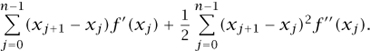
(Of course, now we are assuming that the second derivative f ″ exists and is continuous.) Notice that in the example f(x) = x2 just considered, f″(x) = 2 for every x, and so if we add up all the above approximations we get exactly the right answer. In general, as this observation would suggest, one can show that f(xn) - f(x0) is well-approximated by
Now let us think about what happens to these two sums if we allow our random walks to converge to a Brownian motion Bt. A relatively straightforward argument, based on the fact that (xj+1 - xj)2 is just the reciprocal of the number of steps, shows that the limiting distribution of the second sum exists and is given by the integral ![]() f″ (Bs) ds. This suggests that the first sum should also converge to a limit, which indeed it does: the limit is called the stochastic integral and is written
f″ (Bs) ds. This suggests that the first sum should also converge to a limit, which indeed it does: the limit is called the stochastic integral and is written ![]() f′ (Bs) dBs. More precisely, one ends up with the formula
f′ (Bs) dBs. More precisely, one ends up with the formula
![]()
which is known as Itô’s formula. Note the similarity to the fundamental theorem of calculus. The main difference is the extra term involving the second derivative, the so-called Itô term.
Why, one might wonder, is this interesting? If we wish to estimate the difference between two values of a function by integrating its derivative, why not choose a smooth path rather than a very wiggly one? The point, however, is that we are not interested in just one path. For any fixed sample path, the two sides of the above formula are just numbers, but if we think of Bt as a random variable, then they too become random variables. And since both sides are defined for all t ≥ 0, they are actually stochastic processes. So what we are discussing is a way of integrating one stochastic process to produce another.
The reason Itô’s formula is so useful is that stochastic integrals have properties that allow one to prove many facts about them. In particular, if we view the stochastic integral ![]() f′ (Bs) dBs as a collection of random variables indexed by the parameter t, then we have a stochastic process of an especially nice sort called a martingale. A martingale is a stochastic process (Mt)t ≥ 0 with the property that, whenever s ≤ t, the expected value of Mt, conditional on the values of Mr for all r ≤ s, is just Ms.
f′ (Bs) dBs as a collection of random variables indexed by the parameter t, then we have a stochastic process of an especially nice sort called a martingale. A martingale is a stochastic process (Mt)t ≥ 0 with the property that, whenever s ≤ t, the expected value of Mt, conditional on the values of Mr for all r ≤ s, is just Ms.
Brownian motion is a particularly simple kind of martingale, but martingales are much more general because Mt - Ms is not independent of the values of Mr with r ≤ s: all one knows is that the expectation of Mt - Ms, given those values, is zero. Here is an example that illustrates the difference: start running Brownian motion at 0; when it first reaches 1 (if it ever does), continue with Brownian motion but at double the speed (or rather, double the diffusion constant). In this case, the behavior of Mt - Ms certainly depends on what has happened up to s, but its expectation is nevertheless zero.
In a certain sense, the stochastic integral term in Itô’s formula behaves like a Brownian motion “run at a varying speed,” rather like the example just given. The precise result is that there exists another Brownian motion β = (βt)t≥0 such that, for every t ≥ 0,
![]()
This is in fact true for any continuous martingale—not just one given by a stochastic integral—and the relevant time change is a quantity called the quadratic variation of the martingale. Therefore, the graph of a continuous martingale is obtained from that of a Brownian motion by a time-change operation. This is why Brownian motion is such a central example, and why it is important to understand its behavior before going on to deal with more general stochastic processes.
It is straightforward to generalize the previous derivation of Itô’s formula to multidimensional Brownian motion. If x = (x1, . . ., xd) and y = (y1, . . ., yd) belong to ![]() d and are close together, then the first approximation to f(x) - f(y) is now
d and are close together, then the first approximation to f(x) - f(y) is now

where ∂if(y) denotes the ith partial derivative of f, evaluated at y. The vector of partial derivatives at y is usually denoted ∇ f(y). It is called the gradient of f at y (or “grad f” for short). As for the second derivative of f, it naturally generalizes to the Laplacian Δf (for reasons that are explained in SOME FUNDAMENTAL MATHEMATICAL DEFINITIONS [I.3 §5.4]), and we therefore arrive at the formula
![]()
The stochastic integral term is defined formally in terms of one-dimensional stochastic integrals in the obvious way:

Since stochastic integrals are martingales, the stochastic process
![]()
is (under appropriate conditions on f) a martingale. This observation leads to the martingale problem for Brownian motion. To state a martingale problem for a stochastic process (Xt)t≥0 is to give a collection of martingales defined as functionals of this stochastic process—just as Mf above is defined as a certain function of (Bs)s≥0. The martingale problem is said to be well-posed if it characterizes the distribution of the given stochastic process. In the preceding example, the martingale problem is well-posed: if we know nothing about the distribution of the process (Bt)t≥0 apart from the fact that ![]() is a martingale for every (twice continuously differentiable) function f, we can infer that B must be a Brownian motion.
is a martingale for every (twice continuously differentiable) function f, we can infer that B must be a Brownian motion.
Martingale problems play a fundamental role in modern probability theory (see in particular Stroock and Varadhan (1979), and also THE MATHEMATICS OF MONEY [VII.9 §2.3]). The introduction of a suitable martingale problem is often the most convenient way to specify a stochastic process, or more precisely to characterize its probability distribution.
5 Brownian Motion and Analysis
5.1 Harmonic Functions
A continuous function h defined on an open subset U of ![]() d is called harmonic if the average value of h over any closed ball contained in U, or equivalently the average value over the boundary of any such ball, is equal to its value at the center of the ball. A basic result of analysis is that h is harmonic if and only if it is twice continuously differentiable and Δh = 0. Harmonic functions play an important role in several areas of mathematics as well as in physics. For instance, the electrical potential of a conductor in equilibrium is a harmonic function outside the conductor. And if the temperature of the boundary of a body is kept fixed (that is, although different parts of the boundary may have different temperatures, these temperatures do not change over time), then the equilibrium temperature inside the body is also a harmonic function. (See the discussion of the heat equation in the next section.)
d is called harmonic if the average value of h over any closed ball contained in U, or equivalently the average value over the boundary of any such ball, is equal to its value at the center of the ball. A basic result of analysis is that h is harmonic if and only if it is twice continuously differentiable and Δh = 0. Harmonic functions play an important role in several areas of mathematics as well as in physics. For instance, the electrical potential of a conductor in equilibrium is a harmonic function outside the conductor. And if the temperature of the boundary of a body is kept fixed (that is, although different parts of the boundary may have different temperatures, these temperatures do not change over time), then the equilibrium temperature inside the body is also a harmonic function. (See the discussion of the heat equation in the next section.)

Figure 5 The probabilistic solution of the Dirichlet problem.
Harmonic functions have a very close relationship with Brownian motion, which leads to one of the most important connections between probability and analysis. This connection is already apparent from the fact that ![]() , defined in the previous section, is a martingale. It follows from this that h(Bt) is a martingale if (and in fact only if) h is harmonic, since then the second term vanishes. However, we will explain the link between Brownian motion and harmonic functions in a more elementary way, from the classical Dirichlet problem. Let U be a bounded open set, and let g be a continuous real-valued function defined on the boundary ∂U of U. The classical Dirichlet problem is to find a function h that is harmonic on U and is equal to g on the boundary.
, defined in the previous section, is a martingale. It follows from this that h(Bt) is a martingale if (and in fact only if) h is harmonic, since then the second term vanishes. However, we will explain the link between Brownian motion and harmonic functions in a more elementary way, from the classical Dirichlet problem. Let U be a bounded open set, and let g be a continuous real-valued function defined on the boundary ∂U of U. The classical Dirichlet problem is to find a function h that is harmonic on U and is equal to g on the boundary.
The Dirichlet problem has a remarkably simple solution in terms of Brownian motion: take x ∈ U, start a Brownian motion from x, and evaluate g at the point Bτ where this Brownian motion leaves U (see figure 5); then define h(x) to be the average value you get. Why does this work? That is, why is the function h, defined in this way, harmonic, and why does it equal (or, to be more accurate, converge to) g at the boundary?
The answer to the last question is roughly that if x is very close to the boundary, then a Brownian motion started at x is very likely to leave U at a point close to x. Therefore, since g is continuous, the average value of g at the first exit point will be close to the value of g at any point near x.
To show that h is harmonic is more interesting. Let x be a point in U and suppose that the ball of radius r about x is contained in U. We would like to show that h(x) equals the average value of h on the boundary of this ball. Now h(x) is the average value of g at the point where a Brownian motion that starts at x leaves U. Let us work out this average by conditioning on the first point BT where the Brownian path leaves the ball of radius r (see figure 5). By the rotational invariance of Brownian motion, this point will be evenly distributed around the boundary of this ball. If we reach the boundary at a point y, then the average value of g when the path leaves U (conditioning on this extra information) is h(y), by definition. Therefore, h(x) is indeed the average value of h on the boundary of the ball of radius r.
Convincing though this argument might seem, there is a subtlety concealed within it, connected with the fact that a Brownian path will typically cross the boundary of the ball many times. Suppose we tried a similar argument, but this time we conditioned on the value at the last point where the path left the ball. If this point was y, we could not then say that the expected value of g where the path first reached the boundary of U was h(y) because from that point onward the path would be forbidden to enter the ball again, and would therefore not be a Brownian motion.
Recall that the Markov property of a Brownian motion states that, given a fixed time T and another time t with T < t, the value of Bt - BT is independent of Bs for s ≤ T. It may seem that we are applying this principle in the argument above, taking T to be the first time that the Brownian motion reaches the boundary of the ball. But if we do that, then T is not a fixed time since it depends on the Brownian motion. However, the argument can still be made to work because T is a so-called stopping time. Informally, this means that T does not depend on what the Brownian motion does after T. (Therefore the last time it leaves the ball of radius r is not a stopping time, because whether or not a given time is this last time depends on the subsequent behavior of the Brownian motion.) Brownian motion can be shown to have the strong Markov property, which is like the usual Markov property except that T is allowed to be a stopping time. Given this fact, it is not hard to show rigorously that h is harmonic.
5.2 The Heat Equation
Let f be a function on ![]() d (which we shall assume to be continuous and bounded). If we think of f as a temperature distribution at time 0, then the HEAT EQUATION [III.36] models what happens to the temperature at subsequent times. To find a solution to this equation with initial value f means to find a continuous function u(t, x), defined for every t ≥ 0 and x ∈
d (which we shall assume to be continuous and bounded). If we think of f as a temperature distribution at time 0, then the HEAT EQUATION [III.36] models what happens to the temperature at subsequent times. To find a solution to this equation with initial value f means to find a continuous function u(t, x), defined for every t ≥ 0 and x ∈ ![]() d, that solves the partial differential equation
d, that solves the partial differential equation
![]()
whenever t > 0, and that satisfies the condition u(0, x) = f(x) for every x. (The factor ![]() in this equation is not important but it makes the probabilistic interpretation easier to express.)
in this equation is not important but it makes the probabilistic interpretation easier to express.)
The heat equation also has a simple solution in terms of Brownian motion: u(t, x) is defined to be the expected value of f(Bt) when Bt is a Brownian motion that starts at x. This tells us that heat propagates like a collection of infinitesimal Brownian particles.
The preceding probabilistic representation is quite easy to derive since one can write down an explicit formula for the expectation of f(Bt) in terms of the Gaussian density function. Given this formula, all we have to do is differentiate it and check that the equation is satisfied. However, the connection between Brownian motion and the heat equation is much deeper, and in many other cases there is a probabilistic representation for a solution but no explicit formula. To take one example, suppose that we want to solve the heat equation in an open set U with Dirichlet boundary conditions. This means that we specify an initial value f(x) for the temperature of each point x ∈ U and stipulate that the temperature at the boundary is kept at 0. In other words, we want to find a function u(t, x) such that u(0, x) = f(x) for every x ∈ U, u(t, x) = 0 for every time t ≥ 0 and every x in the boundary of U, and u satisfies the heat equation inside U. In this case, the solution is obtained as follows. Run a Brownian motion (Bt) starting at x. Let gt = f(Bt) if it has not left U at any time before t, and let gt = 0 otherwise. Then define u(t, x) to be the expected value of gt.
Thus, in order to obtain the solution, we had to make just a small modification to the solution of the heat equation in ![]() d. An analytic treatment of this version of the heat equation would be much more complicated.
d. An analytic treatment of this version of the heat equation would be much more complicated.
5.3 Holomorphic Functions
Let us now concentrate on the case d = 2. As usual, we identify ![]() 2 with the complex plane
2 with the complex plane ![]() . Let f = f1 + if2 be a HOLOMORPHIC FUNCTION [I.3 §5.6] defined on
. Let f = f1 + if2 be a HOLOMORPHIC FUNCTION [I.3 §5.6] defined on ![]() . Then the real part f1 and the imaginary part f2 of f are both harmonic functions, so that f1(Bt) and f2(Bt) are martingales. More precisely, Itô’s formula tells us that, for j = 1, 2,
. Then the real part f1 and the imaginary part f2 of f are both harmonic functions, so that f1(Bt) and f2(Bt) are martingales. More precisely, Itô’s formula tells us that, for j = 1, 2,
![]()
since the Itô term vanishes. As we saw in section 3, each of the two processes fj(Bt) can be expressed as a time change of a linear Brownian motion βj. However, a stronger result can also be proved, namely that the time change is the same in both cases and that the Brownian motions β1 and β2 are independent. This makes it possible to prove a “localized” rotational invariance, which leads to the important conformal invariance property of Brownian motion. Roughly speaking, this states that the image of a planar Brownian motion under a conformal (that is, angle-preserving) mapping is another planar Brownian motion run at a different speed.
6 Stochastic Differential Equations
Imagine a Brownian particle in some water. If the temperature of the water rises, then we expect there to be more collisions with faster-moving molecules; this can be modeled easily by increasing the diffusion constant. But what if the temperature in the water varied from place to place? Then the particle would be more agitated in some parts of the water than in others. And if the water was moving, with different parts moving at different speeds, then one would need to superimpose on the Brownian motion a “drift” term, to take into account that on average we would expect the particle to move with the surrounding water.
Stochastic differential equations are used to model more complicated situations like this. Let us begin by considering the one-dimensional case. Let σ and b be two functions (which we shall assume to be continuous) defined on ![]() . We think of σ(x) as telling us the rate of diffusion at x and of b(x) as the drift at x. (For the sake of a picture, one could think of σ(x) as the local temperature at x and b(x) as the velocity at x of some “one-dimensional water.”) Let (Bt) be a one-dimensional Brownian motion.
. We think of σ(x) as telling us the rate of diffusion at x and of b(x) as the drift at x. (For the sake of a picture, one could think of σ(x) as the local temperature at x and b(x) as the velocity at x of some “one-dimensional water.”) Let (Bt) be a one-dimensional Brownian motion.
The notation used for the associated stochastic differential equation is
![]()
Here (Xt) is an unknown stochastic process. The idea is that, infinitesimally speaking, its behavior is like that of a Brownian motion with diffusivity σ(Xt) (which is the diffusivity at the point that Xt has reached) superimposed onto a linear motion at speed b(Xt). More precisely, a solution to the above equation is defined to be a continuous stochastic process (Xt) that satisfies, for every t ≥ 0, the integral equation
![]()
Notice that if σ(x) = 0 for every x, this boils down to the ordinary differential equation x′ (t) = b(x(t)). The stochastic integral ![]() σ(Xs) dBs is defined by approximations similar to those described in section 4. (For this to work, there are certain technical conditions that the process (Xt) must satisfy.) In fact, stochastic differential equations were Itô’s original motivation for developing stochastic integrals.
σ(Xs) dBs is defined by approximations similar to those described in section 4. (For this to work, there are certain technical conditions that the process (Xt) must satisfy.) In fact, stochastic differential equations were Itô’s original motivation for developing stochastic integrals.
Itô proved, under suitable conditions on σ and b, that for each x ∈ ![]() the above equation has a unique solution (Xt) that starts at x. Furthermore, this solution is a Markov process in the sense that was explained above: the way that (Xt) evolves after time T given the value of XT is independent of what happens before T, and is distributed in the same way as a solution of the equation that starts at XT. In fact, it is also a strong Markov process in the sense explained in section 5.
the above equation has a unique solution (Xt) that starts at x. Furthermore, this solution is a Markov process in the sense that was explained above: the way that (Xt) evolves after time T given the value of XT is independent of what happens before T, and is distributed in the same way as a solution of the equation that starts at XT. In fact, it is also a strong Markov process in the sense explained in section 5.
An important example can be found in the famous BLACK-SCHOLES MODEL [VII.9 §2] of mathematical finance. In this model, the price of a share solves a stochastic differential equation of the type above with σ(x) = σx and b(x) = bx, where σ and b are positive constants. This is motivated by the simple idea that the price fluctuations of a share should be roughly proportional to its current value. In this context, the number σ is called the volatility of the share.
The previous discussion generalizes fairly easily to stochastic differential equations in higher dimensions. The solution of a d-dimensional stochastic equation (which when d = 3 could model the water example mentioned at the beginning of this section) is once again a strong Markov process, known as a diffusion process. Much of what was said earlier about the relationship between Brownian motion and partial differential equations can be generalized to diffusion processes as well. Roughly speaking, with each diffusion process one can associate a differential operator L, and this operator plays the role that the Laplacian plays for Brownian motion.
7 Random Trees
Brownian motion and more general diffusion processes appear as limits of many discrete models in probability theory, combinatorics, and statistical physics. The most striking recent example of this is given by the so-called stochastic Loewner evolution (commonly abbreviated to SLE) processes, which are discussed in [IV.25 § 5]). These are expected to describe the asymptotic behavior of a large number of two-dimensional models, and their definition involves both linear Brownian motion and the Loewner equation from complex analysis. Rather than trying to give a general presentation of the relationship between Brownian motion and discrete models, in this final section we shall discuss a surprising application of Brownian motion to random trees, which can be used to describe the genealogy of a population.
The basic discrete model is the following. We start with a single “ancestor,” which we label ∅. Then we place a probability distribution μ on the nonnegative integers, and use this to determine the number of children the ancestor has. Then each child is assumed to have children, the numbers of children being independent and also determined by the probability distribution μ. And so on. The case that we shall be interested in is the so-called critical case, where the expected number of children is exactly 1 (and the variance is finite).
We can represent the outcome of this process as a labeled tree, called the genealogical tree, in a natural way. To draw the tree one simply joins each member of the population to its children. As for the labels, the children of the original ancestor are labeled 1, 2, . . ., left to right, the children of 1 are labeled (1, 1), (1, 2), . . ., the children of 2 are labeled (2, 1), (2, 2), . . ., and so on. (For instance, the children of (3, 4, 2), if it is ever born, are labeled (3, 4, 2, 1), (3, 4, 2, 2), . . . .) See the left-hand side of figure 6 for a simple example of a tree. It is known that in this critical case the population will eventually die out with probability 1. (To avoid the certainty of this fate, the average number of children must be more than 1. A particular case of this process is discussed in [IV.25 §2].)
The genealogical tree, which we shall denote by θ, is a random variable. It is called the Galton–Watson tree with offspring distribution μ. A convenient way to represent this tree is via its so-called contour function, which is illustrated on the right-hand side of figure 6. Informally, we imagine the motion of a particle that starts from the root and explores the tree from the left to the right, moving continuously along the edges at constant vertical speed (we set the height of each edge to 1), until it has completely explored the tree and come back to its starting point, after which it stays at this point. Since the particle will go along each edge exactly twice in this evolution, once upward and once downward, the total time T(θ) needed to explore the tree is twice the number of edges. The value ![]() of the contour function at time t is the height of the particle at time t. All this should be clear from figure 6.
of the contour function at time t is the height of the particle at time t. All this should be clear from figure 6.

Figure 6 Left: a tree θ. Right: the contour function Cθ.
It may be that a typical tree dies out fairly quickly. However, our goal is to understand the shape of the tree when it is “conditioned to be large.” This is a bit like the difference between on the one hand picking a random person alive one thousand years ago and looking at the tree of all his or her descendants, and on the other hand looking at the tree of a random ancestor, alive one thousand years ago, of an individual who is alive today. In the latter case the tree is guaranteed to continue for many generations without dying out.
Suppose we condition on the event that the tree θ (or rather the population it represents) survives for n generations. We may now ask all sorts of questions about this genealogical tree. How many individuals are there in a given generation of the tree? If we pick two individuals in the same generation, how far do we typically have to go back in the tree to reach a common ancestor? Asymptotic answers to such questions are also of interest in computer science and in combinatorics.
We will condition on a slightly different event, namely the event that θ has exactly n edges. The conditioned tree is called θn. It is a random tree with n edges, so T(θn) = 2n.
In the particular case where the probability μ(k) of having k children is 2-(k+1), it is not hard to prove that the distribution of θn will actually be uniform over all trees with n edges. A famous theorem of Aldous gives the asymptotic behavior of the contour function Cθn as n → ∞ for general offspring distributions, and it turns out to be very closely related to a linear Brownian motion.
Notice that it cannot be a Brownian motion because it exhibits some behavior that is very untypical: it begins and ends at zero and remains positive for all time. However, we can use Brownian motion in a simple way to define a notion called a Brownian excursion, for which the sample paths have the right shape. The rough idea is to start a linear Brownian motion at zero, draw its graph, and then pick out the part of the graph between x = x1 and x = x2, where x1 is the point where it last crosses the x-axis before x = 1 and x2 is the point where it first crosses the x-axis after x = 1. The corresponding portion of the Brownian motion will start and end at zero and not cross zero in between. We then need to rescale it so that x goes from 0 to 1 instead of from x1 to x2, and we also need to rescale the height appropriately, by dividing by 1/![]() . Also, if the path is everywhere negative between x1 and x2, we simply turn it upside down to make it positive.
. Also, if the path is everywhere negative between x1 and x2, we simply turn it upside down to make it positive.
Aldous’s theorem states that the limiting distribution of the contour function Cθn (rescaled in time by the factor 1/2n and in space by the factor 1/![]() , like the rescaling in section 3) is a Brownian excursion. The surprising fact about this result is that it does not depend on the offspring distribution μ. Since the contour function completely determines the shape of the corresponding tree, we find that the limiting shape of a large critical Galton–Watson tree does not depend on the offspring distribution. This is another example of universality.
, like the rescaling in section 3) is a Brownian excursion. The surprising fact about this result is that it does not depend on the offspring distribution μ. Since the contour function completely determines the shape of the corresponding tree, we find that the limiting shape of a large critical Galton–Watson tree does not depend on the offspring distribution. This is another example of universality.
This result and variants of it provide a lot of useful information about the asymptotic behavior of large trees. Many interesting functions of the tree can be rewritten in terms of the contour function and by Aldous’s theorem they will converge to similar functions of the Brownian excursion, whose distribution can be computed explicitly with the help of stochastic calculus. To give just one example, this technique can be used to calculate the limiting distribution of the height of the tree θn. Let the variance of the offspring distribution be σ, and let us define the rescaled height of a tree to be its original height multiplied by σ/2![]() . The probability that this is at least x turns out to converge, as n gets large, to the quantity
. The probability that this is at least x turns out to converge, as n gets large, to the quantity

Acknowledgments. The author is indebted to Gilles Stoltz for his help with the simulations and to Gordon Slade for his remarks on the first version of this article.
Further Reading
Aldous, D. 1993. The continuum random tree. III. Annals of Probability 21:248–89.
Bachelier, L. 1900. Théorie de la spéculation. Annales Scientifiques de Ì’École Normale Supérieure (3) 17:21–86.
Billingsley, P. 1968. Convergence of Probability Measures. New York: John Wiley.
Durrett, R. 1984. Brownian Motion and Martingales in Analysis. Belmont, CA: Wadsworth.
Einstein, A. 1956. Investigations on the Theory of the Brownian Movement. New York: Dover.
Revuz, D., and M. Yor. 1991. Continuous Martingales and Brownian Motion. New York: Springer.
Stroock, D. W., and S. R. S. Varadhan. 1979. Multidimensional Diffusion Processes. New York: Springer.
Wiener, N. 1923. Differential space. Journal of Mathematical Physics Massachusetts Institute of Technology 2:131–74.