
IV.18 Enumerative and Algebraic Combinatorics
Doron Zeilberger
1 Introduction
Enumeration, otherwise known as counting, is the oldest mathematical subject, while algebraic combinatorics is one of the youngest. Some cynics claim that algebraic combinatorics is not really a new subject but just a new name given to enumerative combinatorics in order to enhance its (former) poor image, but algebraic combinatorics is in fact the synthesis of two opposing trends: abstraction of the concrete and concretization of the abstract. The former trend dominated the first half of the twentieth century, starting with Hilbert’s “theological” proof of the fundamental theorem of invariants, in which he showed by abstract means that certain invariants existed, but not how to find them. The latter trend is dominating contemporary mathematics, thanks to the omnipresence of The Mighty Computer.
The abstraction trend consists of the categorization, conceptualization, structuralization, and fancification (in short, “BOURBAKIZATION” [VI.96]) of mathematics. Enumeration did not escape this trend, and in the hands of such giants as Gian-Carlo Rota and Richard Stanley in America and Marco Schützenberger and Dominique Foata in France, classical, enumerative combinatorics became more conceptual, structural, and algebraic. However, as algebraic combinatorics has established itself as a fully fledged and separate mathematical speciality, the more recent trend toward the explicit, concrete, and constructive has left its mark as well. It has revealed that many algebraic structures have hidden combinatorial underpinnings; the attempts to unearth these have led to many fascinating discoveries and unsolved problems.
1.1 Enumeration
The fundamental theorem of enumeration, independently discovered by several anonymous cave dwellers, states that
![]()
In words: the number of elements in A is the sum over all elements of A of the constant function 1.
While this formula is still useful after all these years, enumerating specific finite sets is no longer considered mathematics. A genuine mathematical fact has to incorporate infinitely many facts, and the generic enumeration problem is to enumerate not just one set but all the sets in an infinite family.
To be precise, given an infinite sequence of sets ![]() , where each set An consists of objects satisfying some combinatorial specifications that depend on the parameter n, answer the question: How many elements does An have?
, where each set An consists of objects satisfying some combinatorial specifications that depend on the parameter n, answer the question: How many elements does An have?
In a moment we shall look at some examples. But before we can learn how to answer this kind of question, let us consider a meta-question: What is an answer?
This was posed, and beautifully answered, by Herbert Wilf. To give some background to Wilf’s meta-answer, let us examine answers to some famous instances of enumeration questions.
In the list below, when we are given a set An (which will change from example to example), we shall write an instead of |An|. That is, an will stand for the number of elements of An.
(i) I Ching. If An is the set of all subsets of {1, . . . , n}, then an = 2n.
(ii) Rabbi Levi Ben Gerson. If An is the set of PERMUTATIONS [III.68] on {1, . . . , n}, then an = n!.
(iii) Catalan. If An is the set of legal bracketings with n opening brackets and n closing brackets, then an = (2n)!/(n + 1)!n!. (A legal bracketing is a sequence of n opening brackets and n closing brackets such that at no point in the sequence has the number of closing brackets exceeded the number of opening brackets. For instance, when n = 2 the legal bracketings are [][]and[[]].)
(iv) LEONARDO OF PISA [VI.6]. Let An be the set of finite sequences that consist only of is and 2s and that sum to n. (For example, when n = 4 the possible sequences are 1111, 112, 121, 211, and 22.) In this case, we have three equivalent answers as follows.
(i)
![]()
(ii)

(iii) an = Fn + 1, where Fn is the sequence defined by the recurrence Fn = Fn-1 + Fn-2, subject to the initial conditions F0 = 0, F1 = 1.
(v) CAYLEY [VI.46]. If An is the set of labeled trees on n vertices, then an = nn-2. (A tree is a connected GRAPH [III.34] without cycles, and it is labeled if the vertices have distinct names.)
(vi) If An is the set of labeled simple graphs with n vertices, then an = 2n(n-1)/2. (A graph is simple if it has neither loops nor multiple edges.)
(vii) If An is the set of labeled connected simple graphs on n vertices (that is, graphs for which every vertex can be reached from every other by a path), then an is n! times the coefficient of xn in the power-series expansion of
![]()
(viii) If An is the set of Latin squares of size n (n × n matrices each of whose rows and columns is a permutation of {1, . . . , n}), then not even a good approximation for an is known.
In 1982, Wilf defined an answer as follows.
Definition. An answer is a polynomial-time algorithm (in n) for computing an.
Wilf arrived at this definition after he refereed a paper proposing a “formula” for the answer to question (viii), and realized that its “computational complexity” exceeds that of the caveman’s formula of direct counting.
What is a “formula”? It is really an algorithm that inputs n and outputs an. For example, an = 2n is shorthand for the recursive algorithm
if n = 0 then an = 1,
else an = 2 · an-1,
which takes O(n) steps. However, using the algorithm
if n = 0 then an = 1,
else if n is odd, then an = 2an-1,
else ![]()
takes 0 (log n) steps, much faster than Wilf demands. In other cases, like enumerating self-avoiding walks, the best algorithm known is exponential, O(cn), and any lowering of the constant c is a major advance. (A self-avoiding walk is a sequence of points x0, x1, . . . , xn in the two-dimensional integer lattice, where each xi is one of the four neighbors of xi-1 and no two of the xi are equal.) Notwithstanding these exceptions, Wilf’s meta-answer is a very useful general guideline for evaluating answers.
Traditionally, the main customers of enumeration were probability and statistics. In fact, discrete probability is almost synonymous with enumerative combinatorics, since the probability of an event E occurring is the ratio of the number of successful cases divided by the total number. Also, statistical physics is, by and large, weighted enumeration of lattice models (see PHASE TRANSITIONS AND UNIVERSALITY [IV.25]). About fifty years ago, another important customer came along: computer science. Here one is interested in the COMPUTATIONAL COMPLEXITY [IV.20] of algorithms: that is, in the number of steps it takes to execute them.
2 Methods
The following tools are indispensable to the enumerative combinatorialist.
2.1 Decomposition
|A ∭ B| = |A| + |B| (if A ∩ B = ø).
In words: the size of the union of two disjoint sets equals the sum of their sizes.
|A × B| = |A| · |B|.
In words: the size of the Cartesian product of two sets (that is, the set of all pairs (a, b), where a ∈ A and b ∈ B) equals the product of their sizes.
|AB| = |A||B|.
In words: the size of the set of functions from B to A equals the size of A raised to the power the size of B. For example, the number of 0-1 sequences of length n, which can be viewed as functions from {1, 2, . . . , n} to {0, 1}, equals 2n.
2.2 Refinement
If
![]()
and if bnk, the number of elements of Bnk, is “nice” (and even if it is not), then
![]()
The idea here is that it may be possible to take a set An that is difficult to count, and split it up into disjoint sets Bnk that are easier to count. For example, consider the set An of example (iv). This can be split into a disjoint union of subsets Bnk, where each Bnk consists of the sequences in An that have exactly k 2s. If there are k 2s, then there must be n - 2k 1s, so ![]() This yields answer (ii).
This yields answer (ii).
2.3 Recursion
Suppose that An can be decomposed in such a way that it is a combination of fundamental operations applied to the sets An-1, An-2, . . . , A0. Then an satisfies a recurrence relation of the form
an = P(an-1, an-2, . . . , a0).
For example, let An be the set of example (iv). If a sequence in An starts with a 1, then the rest of the sequence must add up to n – 1, and if it starts with a 2, then the rest must add up to n – 2. Since when n ≥ 2 exactly one of these possibilities occurs and both are possible, we can decompose An into lAn-1 and 2An-2, where lAn-1 is shorthand for the set of all sequences that begin with a 1 and continue with a sequence in An-1, and 2An-2 is defined similarly. Since the sizes of lAn-1 and 2An-2 are clearly an-1 and an-2, it follows that an = an-1 + an-2, which yields answer (iii).
If An is the set of legal bracketings with n pairs (example (iii)), then a typical legal bracketing can be written recursively as [L1 ]L2, where L1 and L2 are smaller (possibly empty) legal bracketings. For example, if the bracketing is [ [ ] [ ] ] [ [ ] ] [ [ ] [ [ ] ] ] then L1 = [][] and L2 [ [ ] ] [ [ ] [ [ ] ] ]. If L1 has k pairs, then L2 has n – 1 – k pairs. It follows that An can be identified with the union ![]() and, taking cardinalities,
and, taking cardinalities, ![]() This is a nonlinear (in fact, quadratic) and nonlocal recurrence, but it is nevertheless one that satisfies Wilf’s dictum.
This is a nonlinear (in fact, quadratic) and nonlocal recurrence, but it is nevertheless one that satisfies Wilf’s dictum.
2.4 Generatingfunctionology
According to Wilf, who coined this neologism by making it the title of his classic book (a free download from his Web site, even though it is still in print!):
A generating function is a clothesline on which we hang up a sequence of numbers for display.
The method of generating functions is one of the most useful tools of the trade of enumeration. The generating function of a sequence, sometimes called its z-transform, is a discrete analogue of the LAPLACE TRANSFORM [III.91], and indeed goes back to LAPLACE [VI.23] himself. If the sequence is ![]() then its generating function f(x) is defined to be
then its generating function f(x) is defined to be ![]() In other words, the terms of the sequence are regarded as the coefficients of a power series in x.
In other words, the terms of the sequence are regarded as the coefficients of a power series in x.
Generating functions are so useful because information about the sequence (an) translates to information about f(x) that is often easier to process, and after some manipulations one often gets additional information about f(x) that can be translated back into information about the sequence. For example, if a0 = a1 = 1 and an = an-1 an-2 when n ≥ 2, then we can do the following manipulations on f(x):

It follows that
![]()
If one performs a partial-fraction decomposition, and expands the two resulting terms in a Taylor series, then one can obtain answer (i) to example (iv).
3 Weight Enumeration
According to the modern approach, pioneered by Pólya, Tutte, and Schützenberger, generating functions are neither “generating,” nor are they functions. Rather, they are formal power series that are weight enumerators of combinatorial sets. (Usually, but not always, these sets are infinite: for a finite set the corresponding “power series” has only finitely many nonzero terms and is therefore a polynomial.)
A power series ![]() is called formal when one sheds its analytical connotation as a Taylor series of a function, and thereby obviates the need to worry about convergence. For example, the sum
is called formal when one sheds its analytical connotation as a Taylor series of a function, and thereby obviates the need to worry about convergence. For example, the sum ![]() is perfectly legal as a formal power series even though it converges only when x = 0.
is perfectly legal as a formal power series even though it converges only when x = 0.
As for weight enumerators, consider the following situation. Suppose that we want to study the age distribution of a finite population. One way of doing this is to ask 121 questions. For each i between 0 and 120, we ask those whose age is i to raise their hand. Then we count each of these age-groups one by one, compiling a table of ai (0 ≤ i ≤ 120), and finally computing the generating function
![]()
But if the size of the population is much less than 120, it is much more efficient, because fewer questions would be needed, to ask every person their age and then to declare the weight of a person of age i to be xi. Then the generating function is the sum of these weights. That is,
![]()
which is a natural extension of the caveman’s formula of naive counting. Once we know f(x) we can easily compute statistically interesting quantities, like the average and the variance, which work out to be μ = f′(1)/f(1) and σ2 = f″(1)/f(1)+μ–μ2, respectively.
The general scenario is that we have an interesting (finite or infinite) combinatorial set, let us call it A, and a certain numerical attribute, α : A → ![]() , which assigns to each element of A a natural number. (Here we allow 0 as a natural number.) Then the weight enumerator of A with respect to α is defined by the formula
, which assigns to each element of A a natural number. (Here we allow 0 as a natural number.) Then the weight enumerator of A with respect to α is defined by the formula
![]()
We shall also use the notation |A|x for f(x). Obviously, this equals
![]()
where an is the number of members of A whose α equals n. Hence if we have some kind of explicit expression for f(x), we immediately have an “explicit” expression for the actual sequence αn assuming, that is, that one considers the operations needed to calculate the nth coefficient an of f(x) as constituting an explicit expression for an. Even if one does not, then it is still often possible to get a “nice” formula for an or, failing this, to extract the asymptotics.
The fundamental operations for naive counting also hold for weighted counting: just replace | · | by | · |x. For example,
|A ∪ B|x = |A|x + |B|x
(if A ∩ B = ø) and
|A × B|x = |A|x · |B|x.
Let us quickly see why the second of these is true. If the members of A and B are endowed with numerical attributes α and β, respectively, and one defines an attribute γ on A×B by letting γ (a, b) equal α(a)+β(b), then

Let us see how these facts can be useful. First, consider the infinite set A, of all (finite) sequences of 1s and 2s, and let the attribute be “sum of entries.” Then the weight of 1221 is x6, and, in general, the weight of a sequence (a1 · · · ar) is xa1 + ···+ak. The set A can be naturally decomposed as
A {![]() } ∪ 1A ∪ 2A,
} ∪ 1A ∪ 2A,
where ![]() is the empty word, and 1A is short for the set of all sequences obtained by prefixing a 1 to members of A, and analogously for 2A. Applying | · |x, we get
is the empty word, and 1A is short for the set of all sequences obtained by prefixing a 1 to members of A, and analogously for 2A. Applying | · |x, we get
|A|x = 1 + x|A|x + x2|A|x,
which, in this simple case, can be solved explicitly, to yield, once again
![]()
A legal bracketing L is either empty (in which case the weight is x0 = 1), or else, as we have already noted, it can be written as L = [L1]L2, where L1 and L2 are (shorter) legal bracketings. Conversely, whenever L1 and L2 are legal bracketings, so is [L1]L2. Let L be the (infinite) set of all legal bracketings, and define the weight of a legal bracketing to be xn, where n is the number of bracket pairs [ ]. For example, the weight of [] is x and the weight of [ [ ] [ [ ] [ ] ] ] is x5. The set ![]() decomposes naturally as follows:
decomposes naturally as follows:
![]() = {
= {![]() } ∪ ([
} ∪ ([![]() ] ×
] × ![]() ),
),
where ![]() denotes the empty word and [
denotes the empty word and [![]() ] ×
] × ![]() denotes the set of all words of the form [
denotes the set of all words of the form [![]() 1]
1]![]() 2 with
2 with ![]() 1 and
1 and ![]() 2 in
2 in ![]() . This leads to the nonlinear (in fact, quadratic) equation
. This leads to the nonlinear (in fact, quadratic) equation
![]()
which yields, thanks to the Babylonians, the explicit expression
![]()
This in turn gives us the answer to example (iii) above, via Newton’s binomial theorem.
Legal bracketings are equivalent to so-called binary trees, that is, unlabeled ordered trees where every vertex has either no children or exactly two children. For instance, when we write the legal bracketing [ [ ] [ ] ] [ [ ] ] [ [ ] [ [ ] ] ] in the form [![]() 1]
1]![]() 2 we can think of [ [ ] [ ] ] [ [ ] ] [ [ ] [ [ ] ] ] as the parent, with children
2 we can think of [ [ ] [ ] ] [ [ ] ] [ [ ] [ [ ] ] ] as the parent, with children ![]() 1 = [ ] [ ] and
1 = [ ] [ ] and ![]() 2 = [ [ ] ] [ [ ] [ [ ] ] ]. Then
2 = [ [ ] ] [ [ ] [ [ ] ] ]. Then ![]() 1’s children are
1’s children are ![]() and [ ], while
and [ ], while ![]() 2’s are [ ] and [ [ ] [ [ ] ] ]. This process continues until we have reached
2’s are [ ] and [ [ ] [ [ ] ] ]. This process continues until we have reached ![]() down every branch of the family.
down every branch of the family.
If we try to count penta-trees instead, where each vertex may only have exactly zero or five children, then the generating function, alias weight-enumerator, satisfies the quintic equation
f = x + f5,
which, according to ABEL [VI.33] and GALOIS [V1.41], is not solvable by radicals (see THE INSOLUBILITY OF THE QUINTIC [V.21]). However, solvability by radicals is not everything. More than 200 years ago, LAGRANGE [VI.22] devised a beautiful and extremely useful formula for extracting the coefficients of the generating function from the equation it satisfies, now called the Lagrange inversion formula. Using it one can easily show that the number of complete k-ary trees with (k–1)m+1 leaves is
![]()
A multivariate generalization of the Lagrange inversion formula, discovered by the great Bayesian probabilist I. J. Good, enables one to enumerate colored trees and many other extensions.
3.1 Enumeration Ansatzes
If one wants to turn enumerative combinatorics into a theory rather than a collection of solved problems, one needs to introduce classification, and enumeration paradigms for counting sequences. But since “paradigm” is such a pretentious word, let us use the much humbler German word “ansatz,” which roughly means “form of solution.”
Let ![]() be a sequence, and let
be a sequence, and let
![]()
be its generating function. If we know the “form” of an, we can often deduce the form of f (x) (and vice versa).
(i) If an is a polynomial in n, then f(x) has the form
![]()
where P is a polynomial function and d is the degree of the polynomial that describes an.
(ii) If an is a quasi-polynomial in n (i.e., there exists an integer N such that for each r = 0, . . . , N – 1, the function m ![]() amN+r is a polynomial in m), then, for some (finite) sequence of integers d1, d2,. . . and some polynomial function P,
amN+r is a polynomial in m), then, for some (finite) sequence of integers d1, d2,. . . and some polynomial function P,
![]()
(iii) If an is C-recursive, that is, if it satisfies a linear recurrence equation with constant coefficients
an = c1an-1 + c2an-2 + · · · + cdan-d
(a good example is the Fibonacci sequence), then f(x) is a rational function of x: that is, f(x) = P(x)/Q(x), where P and Q are polynomials.
(iv) If an satisfies a linear recurrence equation of the form
![]()
where the coefficients ci(n) are polynomial in n, then it is said to be P-recursive. (For example, an = n! is P-recursive since we have the recurrence an = nan-1.) If this is the case, then f(x) is D-finite, which means that it satisfies a linear differential equation with polynomial coefficients (in x).
In the case of an = n! the recurrence an = nan-1 is first order. A natural example of a P-recursive sequence satisfying a higher-order linear recurrence with polynomial coefficients is the sequence that counts the number of involutions on {1, . . . , n}. (An involution is a permutation that equals its inverse.) Let us call this number wn. The sequence (wn) satisfies the recurrence relation
wn = wn-1 + (n – 1)wn-2.
This recurrence follows from the fact that in the permutation n belongs either to a 1-cycle or to a 2-cycle. The former case accounts for wn-1 of the involutions, and the latter for (n – 1)Wn-2 of them. (There are n – 1 ways of choosing the cycle-mate, i, say, of n, and deleting the resulting cycle leaves an involution of the n – 2 elements {1, . . . ,i – 1, i+1, . . . ,n – 1}.)
4 Bijective Methods
This last argument was a simple example of a bijective proof, in this case, of a recurrence for the number of involutions on n objects. Contrast it with the following proof.
The number of involutions of {1, . . . , n} with exactly k 2-cycles is
![]()
because we must first choose the 2 k elements that will participate in the k 2-cycles, and then match them up into (unordered) pairs, which can be done in
![]()
ways. Hence
![]()
Nowadays such sums can be handled completely automatically, and if one inputs this sum to the Maple package EKHAD (downloadable from my Web site), one would get the recurrence wn = wn–1 + (n – 1) wn—2 as the output, together with a (completely rigorous!) proof. While the so-called Wilf-Zeilberger (WZ) method is able to handle many such problems, there are many other cases where one still needs a human proof. In either case such proofs involve (algebraic, and sometimes analytic) manipulations. The great combinatorialist Adriano Garsia derogatorily calls such proofs “manipulatorics,” and real enumerators do not manipulate, or at least try to avoid it whenever possible. The preferred method of proof is by BIJECTION [I.2 §2.2].
Suppose one has to prove that |An| = |Bn| for every n, where An and Bn are combinatorial families The “ugly way” is to get, by some means or other, algebraic or analytic expressions for an = |An| and bn = |Bn|. Then one manipulates an, getting another expression ![]() which in turn leads to yet another expression
which in turn leads to yet another expression ![]() and if one is patient enough, and clever enough, and in luck, or if the problem is not too deep, one eventually arrives at bn, and the result follows.
and if one is patient enough, and clever enough, and in luck, or if the problem is not too deep, one eventually arrives at bn, and the result follows.
On the other hand, the nice way of proving that |An| = |Bn| is by constructing a (preferably nice) bijection Tn : An → Bn, which immediately implies, as a corollary, that |An| = |Bn|·
In addition to being more aesthetically pleasing, a bijective proof is also philosophically more satisfactory. In fact, the notion of (cardinal) number is a highly sophisticated derived notion based on the much more basic notion of being in bijection. Indeed, according to FREGE [VI.56], the cardinal numbers are equivalence classes, where the EQUIVALENCE RELATION [I.2 §2.3] is “is in bijective correspondence with.” Saharon Shelah said that people have been exchanging objects, in a one-to-one way, since long before they started to count. Also, a bijective proof explains why the two sets are equinumerous, as opposed to just certifying the formal correctness of this fact.
For example, suppose that Noah had wanted to prove that there were as many male as female creatures in his Ark. One way of proving this would have been to count the males and count the females, and check that the two resulting numbers were indeed the same. But a much better, conceptual, proof would have been to note that there is an obvious one-to-one correspondence between the set M of males and the set F of females: the function w : M → F defined by h (y) = HusbandOf(y) .
A classic example of a bijective proof is Glaisher’s proof of EULER’s [VI.19] “odd equals distinct” partition theorem. A partition of an integer n is a way of writing it as a sum of positive integers, where order does not matter. For example, 6 has eleven partitions: 6, 51, 42, 411, 33, 321, 3111, 222, 2211, 21111, 111111. (Here 3111 is shorthand for the sum 3 + 1 + 1 + 1, and so on. Since order does not matter, we count 3111 as the same partition of 6 as 1311, 1131, and 1113. It is convenient to write the partitions with their numbers in decreasing order, as we have done.)
A partition is called odd if all its parts are odd, and it is called distinct if all its parts are distinct. Let Odd(n) and Dis(n) be the sets of odd and distinct partitions of n, respectively. For example, Odd(6) = {51, 33, 3111, 111111} and Dis(6) = {6, 51, 42, 321}. Euler proved that | Odd(n)| = | Dis(n) | for all n. His “manipulatorics” proof goes as follows. Let o (n) and d(n) be the number of odd and distinct partitions of n, respectively, and let us define the generating functions
![]()
With the help of the “multiplication principle” for weighted counting, Euler showed that
![]()
Using the algebraic identity 1 + y = (1 - y2)/(1 we have

Hence g(q) = f(q), and the identity o(n) = d(n) follows by extracting the coefficient of qn.
For a very long time, these kinds of manipulation were considered to belong to the realm of analysis, and in order to justify the manipulations of the infinite series and products, one talked about the “region of convergence,” usually |q| < 1, and every step had to be justified by the appropriate analytical theorem. Only relatively recently did people come to realize that no analysis need be involved: everything makes sense in the completely elementary and much more rigorous (from the philosophical viewpoint) algebra of formal power series. One still needs to worry about convergence, so as to exclude, for example, an infinite product like ![]() (1 + x), but the notion of convergence in the ring of formal power series is much more user-friendly than its analytical namesake.
(1 + x), but the notion of convergence in the ring of formal power series is much more user-friendly than its analytical namesake.
Even though invoking analysis was a red herring, Euler’s proof, while purely algebraic and elementary, is nevertheless still manipulatorics. It would be much nicer to find a direct bijection between the sets Dis(n) and Odd(n). Such a bijection was given by Glaisher. Given a distinct partition, write each of its parts as 2r · s, where s is odd, and replace it by 2r copies of s. (For example, 12 = 4 · 3, so we would replace 12 by 3 + 3 + 3 + 3.) The output is obviously a partition of the same integer n, but now into odd parts. For example, the partition (10, 5, 4) is transformed to the new partition (5, 5, 5, 1, 1, 1, 1). To define the inverse transformation, take an odd part a and count how many times it shows up. If it shows up m times, then write m in binary notation,![]() and replace the m copies of a by the k parts:
and replace the m copies of a by the k parts: ![]() It is not hard to check that if you do the first transformation to a partition in Dis(n) and then do the second transformation, you get back to the partition you started with.
It is not hard to check that if you do the first transformation to a partition in Dis(n) and then do the second transformation, you get back to the partition you started with.
When we perform algebraic (and logical, and even analytical) manipulations, we are really rearranging and combining symbols, and hence we are doing combinatorics in disguise. In fact, everything is combinatorics. All we need to do is to take the combinatorics out of the closet, and make it explicit. The plus sign turns into (disjoint) union, the multiplication sign becomes Cartesian product, and induction turns into recursion. But what about the combinatorial counterpart of the minus sign? In 1982, Garsia and Steven Milne filled this gap by producing an ingenious “involution principle” that enables one to translate the implication
a = b and c = d ![]() a-c=b-d
a-c=b-d
into a bijective argument, in the sense that if C ![]() A and D
A and D ![]() B, and there are natural bijections f : A → B and g : C → D establishing that |A| = |B|, and |C| = |D|, then it is possible to construct an explicit bijection between A C and BD. Let us define it in terms of people. Suppose that in a certain village all the adults are married, with the result that there is a natural bijection from the set of married men to the set of married women, m
B, and there are natural bijections f : A → B and g : C → D establishing that |A| = |B|, and |C| = |D|, then it is possible to construct an explicit bijection between A C and BD. Let us define it in terms of people. Suppose that in a certain village all the adults are married, with the result that there is a natural bijection from the set of married men to the set of married women, m ![]() WifeOf (m), with its inverse w
WifeOf (m), with its inverse w ![]() HusbandOf(w). In addition, some of the people have extramarital affairs, but only one per person, and all within the village. There is a natural bijection from the set of cheating men to the set of cheating women, called m MistressOf(m), with its inverse w → LoverOf (w). It follows that there are as many faithful men as there are faithful women. But how do we match them up? (One might imagine, for example, that each faithful man wants a faithful woman to go to church with him)
HusbandOf(w). In addition, some of the people have extramarital affairs, but only one per person, and all within the village. There is a natural bijection from the set of cheating men to the set of cheating women, called m MistressOf(m), with its inverse w → LoverOf (w). It follows that there are as many faithful men as there are faithful women. But how do we match them up? (One might imagine, for example, that each faithful man wants a faithful woman to go to church with him)
Here is how it is done. A faithful man first asks his wife to come with him If she is faithful, she agrees. If she is not, she has a lover, and that lover has a wife. So she tells her husband: “Sorry, hubby, I am going to the pub with my lover, but my lover’s wife may be free.” If this happens, then the man asks the wife of the lover of his wife to go with him, and if she is faithful, she agrees. If she is not he keeps asking the wife of the lover of the woman who has just rejected his proposal. Since the village is finite, he will eventually get to a faithful woman.
The reaction of the combinatorial enumeration community to the involution principle was mixed. On the one hand it had the universal appeal of a general principle, one that should be useful in many attempts to find bijective proofs of combinatorial identities. On the other hand, its universality is also a major drawback, since involution-principle proofs usually do not give any insight into the specific structures involved, and one feels a bit cheated. Such a proof answers the letter of the question, but it misses its spirit. Given a proof of this kind, one still hopes for a really natural, “involution-principle-free proof.” This is the case, for instance, with the celebrated Rogers–Ramanujan identity, which states that the number of partitions of an integer into parts that leave remainder 1 or 4 when divided by 5 equals the number of partitions of that integer with the property that the difference between any two parts is at least 2. For example, if n = 7 the cardinalities of {61, 4111, 1111111} and {7, 61, 52} are the same. Garsia and Milne invented their notorious principle in order to give a Rogers–Ramanujan bijection, thereby winning a $50 prize from George Andrews. However, finding a really nice bijective proof is still an open problem.
A quintessential example of a bijective proof is Prüfer’s proof of CAYLEY’s [VI.46] celebrated result that there are nn-2 labeled trees on n vertices (example (v) earlier). Recall that a labeled tree is a labeled connected simple graph without cycles. Every tree has at least two vertices with only one neighbor (these are called leaves). A certain mapping called the Prüfer bijection associates with every labeled tree T a vector of integers (a1 , . . . ,an–2), with 1 ≤ ai ≥ n for each i . This vector is called its Prüfer code. Since there are nn-2 such vectors, Cayley’s formula follows once we have defined the mapping f : Trees → Codes and proved that it is indeed a bijection. This really needs four steps: defining f, defining its alleged inverse map g, and proving that g o f and f o g are the identity maps on their respective domains.
The mapping f is defined recursively as follows. If the tree has 2 vertices, then its code is the empty sequence. Otherwise, let al be the (sole) neighbor of the smallest leaf and let (a2, . . . , an-2) be the code of the smaller tree obtained by deleting that leaf.
5 Exponential Generating Functions
So far, when we have discussed generating functions, we have been talking about ordinary generating functions (or OGFs). These are ideally suited for counting ordered structures like integer partitions, ordered trees, and words. But many combinatorial families are really sets, where the order is immaterial. For these the natural concept is that of an exponential generating function (or EGF).
The EGF of a sequence ![]() is defined to be
is defined to be

Labeled objects can be often viewed as sets of smaller irreducible objects. For example, a permutation is the disjoint union of cycles, a set partition is the disjoint union of nonempty sets, a (labeled) forest is the disjoint union of labeled trees, and so on.
Suppose that we have two combinatorial families A and B, and suppose that there are a(n) labeled objects of size n in the A family, and b(n) in the B family. We can construct a new set of labeled objects C = A × B, where the labels are disjoint and distinct, and define the size of a pair to be the sum of the sizes of the components. We have
![]()
since we must
(i) decide the size of the first component, k (an integer between 0 and n), which forces the size of the second component to be n - k,
(ii) decide which of the n labels go to the first component (![]() ways), and
ways), and
(iii) pick the objects for each component from the A and B families, respectively, using the available labels (a(k)b(n - k) ways).
Multiplying both sides by xn/n! and summing from n = 0 to n = ∞ yields

Hence EGF(C) = EGF(A) EGF(B). Iterating, we get
EGF(A1 × A2 × . . . × Ak) = EGF(A1) . . . EGF(Ak).
In particular, if all the A i are the same, we have that the EGF of ordered k-tuples, Ak, equals [EGF(A)]k. But if “order does not matter,” then the EGF of k -sets of A- objects is [EGF(A)]k/k!, since there are exactly k! ways of arranging a k-set into an ordered array (since all labels are distinct, all these objects are different). Summing from k = 0 to k = ∞ we get the “fundamental theorem of exponential generating functions.”
If B is a labeled combinatorial family that can be viewed as sets of “connected components” that belong to a combinatorial family A, then
EGF(B) = exp[EGF(A)].
This useful theorem was part of the physics folklore for many years, and was also implicit in many older combinatorial proofs. However, it was explicated only in the early 1970s. It was fully “categorized” by means of Joyal’s theory of species, which grew to be a beautiful theory of enumeration in the hands of the école Québecoise (the Labelle and Bergeron frères, Leroux, and others).
Here are some venerable examples. Let us try to find the EGF of set partitions. That is, let us try to figure out an expression for

where b(n) (so-called Bell numbers) denotes the number of set partitions of an n-element set.
Recall that a set partition of a set A is a set of pairwisedisjoint nonempty subsets of A, {A1, . . . , Ar}, such that the union of all the A i equals A. For example, the set partitions of the 2-element set {1, 2} are {{1}, {2}} and {{1, 2}}.
The atomic objects in this example are nonempty sets. (We think of a set A as being the “trivial” partition of itself into just one set.) Let a(n) be the number of ways of partitioning a set of size n into one nonempty set. Clearly, when n = 0 this cannot be done, so a(0) = 0. When n ≥ there is exactly one way of doing it, so the EGF of the sequence c(n) is
![]()
It follows immediately from the fundamental theorem that

an identity of Bell. Nowadays, with computer algebra systems, this can be used immediately to crank out the first 100 terms of the sequence b(n). For example, in Maple one simply types
taylor(exp(exp(x)-l) ,x=O,101) ;
so this is definitely an answer in the Wilfian sense. We can also easily derive recurrences (albeit ones that need at least 0(n) memory), by differentiating both sides of (1) and comparing coefficients.
That was really easy, so let us go on and prove something much deeper. How about an EGF-style proof of Levi Ben Gerson’s celebrated formula for the number of permutations on n objects, n! (example (ii) earlier)? Every permutation can be decomposed into a disjoint union of cycles, so the atomic objects are now cycles. How many n-cycles are there? The answer is of course (n – 1)!, since (a1, a2, . . . , an) is the same as (a2, a3 , . . . ,an a1), which is the same as (a3 , . . . , an ,a1 ,a2), which means that we can pick the first entry arbitrarily, after which we have (n – 1)! choices for placing the remaining entries. The EGF for cycles is therefore

Using the fundamental theorem, we get that the EGF of permutations is
![]()
and voilà we have a beautiful new proof that the number of permutations on n objects is n!.
This argument may not look very impressive. But a slight modification leads immediately to the (ordinary) generating function for the number of permutations on {1, . . . , n } with exactly k cycles, which we shall denote by c (n, k). Here we are fixing n and letting k vary, so the generating function is ![]() All we have to do to calculate this is go from naive counting to weighted counting, and assign to each permutation the weight α#cycles The fundamental theorem of exponential generating functions carries over word-for- word to weighted counting. The weighted EGF for cycles is α log(1 – x)-1, so the weighted EGF for permutations is
All we have to do to calculate this is go from naive counting to weighted counting, and assign to each permutation the weight α#cycles The fundamental theorem of exponential generating functions carries over word-for- word to weighted counting. The weighted EGF for cycles is α log(1 – x)-1, so the weighted EGF for permutations is
![]()
where
(α)n = α(α + 1) . . . (α + n - 1)
is the so-called rising factorial. We have therefore derived the far less trivial result that the number of permutations of {1, . . . , n} with exactly k cycles equals the coefficient of αk in (α)n.
About ten years ago (Ehrenpreis and Zeilberger 1994) I used this technique to give a combinatorial proof of the Pythagorean theorem in the form
sin2 z + cos2 z = 1.
The functions sin z and cos z are the weighted EGFs for increasing sequences of odd and even lengths, respectively, with weight (-1)[legth/2]. Hence the left-hand side is the weighted EGF for ordered pairs of increasing sequences
a1 < . . . < ak < b1 · · · < br,
such that k and r have the same parity, the sets {al · · · , ak} and {bl, · · · , br} are disjoint, and the union of the two sets is {1, 2, · · · , k + r}. There is a killer involution on these sets of pairs defined as follows.
If ak < br then map the pair to
a1<· · · < ak < br, bl < · · · <br-1
and otherwise map it to
al < · · · < ak-l, bl < · · · < br < ak.
For example, the pair
1,3,5,6 2, |
4, 7, 8, 9, 10, 11, 12, |
whose sign is (-1)2 · (-1)4 = 1, goes to the pair
1, 3, 5, 6, 12 2, |
4, 7, 8, 9, 10, 11, |
whose sign is (-1)2 · (-1)3 = -1 (and vice versa).
Since this mapping changes the sign, and is an involution, all such pairs can be paired up into mutually canceling pairs. But this mapping is undefined for one special pair, namely the pair (empty, empty), whose weight is 1. Therefore, the EGF for the sum of the weights of all pairs is 1, which explains the right-hand side.
Yet another application of this method is a proof of André’s generating function for the number of up- down permutations. A permutation of al · · · an is called up–down (or sometimes zigzcig) if al < a2 > a3 < a4 > a5 < · · · . Let an be the number of up-down permutations. Then
![]()
This is equivalent to saying that

Can you find the appropriate set and the killer involution?
6 Pólya-Redfield Enumeration
Often in enumeration it is easy enough to count labeled objects, but what about unlabeled ones? For example, the number of labeled (simple) graphs on n vertices (example (vi)) is trivially 2n(n-1)/2, but how many unlabeled graphs are there on n vertices? This is much harder, and in general there are no “nice” answers, but the best known way is via a powerful technique initiated by Pólya, which was largely anticipated by Red- field. Pólya enumeration lends itself very efficiently to counting chemical isomers, since, for example, all the carbon atoms “look the same.” Indeed, counting isomers was Pólya’s initial motivation (see MATHEMATICS AND CHEMISTRY [VII.1 §2.3]).
The main idea is to view unlabeled objects as equivalence classes of easy-to-count labeled objects, and to count these equivalence classes. But what is the equivalence? The answer is that there is always a SYMMETRY GROUP [I.3 §2.1] involved, and it leads to a natural equivalence relation. Let the symmetry group be G, and let the set of labeled objects be A. Then two objects a and b of A are regarded as equivalent if b = g(a) for some member g of the group G. This means that there is some symmetry g in the group G that transforms a to b. This is easily seen to be an equivalence relation and the equivalence classes are the sets
Orbit(a) {g(a) | g λ G}, a λA,
which are known as orbits. Calling each orbit a “family,” we have the task of counting the number of families Note that G is a subgroup of the group of permutations of the finite set A.
Suppose that there is a picnic consisting of many families and we want to count the number of families One way would be to define some “canonical head” of each family, say “mother,” and count the number of mothers. But some daughters look like mothers, so this is not so easy. On the other hand, you cannot just count everybody, since then you would count each family several times. The problem is that “naive” counting of people (or objects) is giving a credit of 1 to each person, and this is inappropriate if we are trying to count families. If instead we were to ask each person “How big is your family?” and add to our count the reciprocal of that number, then the calculation would come out just right, since a family of size k would get a credit of 1/k for each of its members, and would therefore have been counted exactly once by the end. Going back to counting orbits, we see by the same reasoning that their number is

The conceptual opposite of “orbit of a” is the subgroup of members of G that fix a:
![]()
(This is sometimes known as the stabilizer of a.) To each element b = ga in the orbit of a, we can associate the left coset g Fix(a) of Fix(a). This association turns out to be a well-defined one-to-one correspondence between the orbit of a and the cosets of Fix(a) in G, from which it follows that the size of Orbit(a) is | G/ Fix(a)|. We can therefore substitute |Fix(a)| / | G| for 1 / | Orbit(a) | in the previous formula, which implies that the number of orbits is
![]()
Let us use the notation χ(statement) to stand for 1 if the statement is true and 0 if it is false. Then

where fix(g) is the number of fixed points of g (when g is viewed as a permutation of A). We have just proved what used to be called Burnside’s lemma, but it goes back to CAUCHY [VI.29] and FROBENIUS [VI.58]. It states that the total number of orbits equals the average number of fixed points of g, over all transformations g in G. If the group G is the full symmetric group of all the permutations of A, then the average number of fixed points equals 1 (since in this trivial case there is only one orbit!).
Enter Pólya. The objects that he was interested in counting (e.g., chemical isomers, or colorings of the faces of the cube) were all naturally functions from an underlying set to a set of colors (or atoms). Let us call the underlying set U and the set of colors C. A symmetry of U gives rise in a natural way to a transformation of the set of functions f : U → C. Given a function f one defines a new function gf by g(f)(u) = f (g (u)). (If we think of f as a coloring, then g f is the new coloring that assigns to u the color that f assigned to g(u).) Now let us think about the number of fixed points of g in the set of C-colorings of U. Such a fixed point is a coloring f that equals gf: that is, f (u) = f(gu) for every u. But then f (u) = f(gu) = f(g2u) = • • • , which means that, given any cycle of g, f must assign the same color to all members of that cycle. It follows that the number of fixed colorings of g is ![]() , where c = |C| is the number of colors.
, where c = |C| is the number of colors.
Applying Burnside’s lemma, we may deduce that the number of different colorings of U (up to G-equivalence) is
![]()
since an equivalence class of colorings is simply an orbit of one of the colorings in that class.
Here is a simple application. How many necklaces (without a clasp) are there that consist of p beads (where p is a prime) and that use a different colors? The underlying set is {0, . . ., p - 1}, and the symmetry group is ![]() p, the cyclic group of order p. As usual, regard the elements of the symmetry group as permutations of the set of beads. Since p is a prime, there are p - 1 elements of
p, the cyclic group of order p. As usual, regard the elements of the symmetry group as permutations of the set of beads. Since p is a prime, there are p - 1 elements of ![]() p with one cycle (of length p), and one element (the identity permutation) with p cycles (all of length 1). It follows that the number of necklaces is
p with one cycle (of length p), and one element (the identity permutation) with p cycles (all of length 1). It follows that the number of necklaces is
![]()
In particular, since this number is necessarily an integer, we get as a bonus a combinatorial proof of FERMAT’S LITTLE THEOREM [III.58]: that ap - a is always a multiple of p. Perhaps one day there will be an equally nice combinatorial proof of Fermat’s last theorem. All one has to do is to prove that there is no bijection from the union of the set of straight necklaces of size n using x colors, and the set of such necklaces using y colors, to the set of necklaces using z colors (with n > 2, of course).
If one wants to keep track of how many beads there are of each color, one simply replaces straight counting by weighted counting, and ![]() is replaced by
is replaced by
![]()
(assuming that g has α1 1-cycles, α2 2-cycles, etc.). The resulting expression is the celebrated cycle-index polynomial.
6.1 The Principle of Inclusion–Exclusion and Möbius Inversion
Another pillar of enumeration is the principle of inclusion–exclusion (nicknamed PIE). Suppose that there are n sins, sl, . . ., sn, that a person may succumb to, and suppose that for each set of sins S, As is the set of people who have all the sins in S (and possibly others). Then the number of good people (without sins) is
![]()
For example, if the set A is the set of all permutations π of {1, . . ., n} and the ith sin is having π [i] = i, then |As| I = (n - |S|)!, and we get that the number of derangements (permutations without fixed points) is
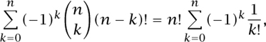
which yields the answer: “closest integer to n!/e.” This is sometimes called the “umbrella problem”: if on a rainy day n absent-minded people go to a party and leave an umbrella by the door, and if on their departure they each take a random umbrella, then the probability that nobody ends up with the right umbrella is about 1/e.
The PIE is a special case of Möbius inversion on general partially ordered sets (posets) where the poset happens to be the Boolean lattice. This realization was published in a seminal paper by Rota (1964) and reprinted in his collected works. It is considered by many to be the big bang that started modern algebraic combinatorics. Möbius’s original inversion formula is recovered when the partially ordered set is ![]() and the partial order is divisibility.
and the partial order is divisibility.
A contemporary account of enumeration from the “algebraic” point of view can be found in a marvelous two-volume set by Stanley (2000), which I strongly recommend.
7 Algebraic Combinatorics
So far I have described one of the routes to algebraic combinatorics: abstraction and conceptualization of classical enumeration. The other route, “concretization of the abstract,” is almost everywhere dense in mathematics, and cannot be described in a few pages. Let me quote from the preface of the excellent New Perspectives in Algebraic Combinatorics by Billera et al. (1999).
Algebraic combinatorics involves the use of techniques from algebra, topology, and geometry in the solution of combinatorial problems, or the use of combinatorial methods to attack problems in these areas. Problems amenable to the methods of algebraic combinatorics arise in these or other areas of mathematics or from diverse parts of applied mathematics. Because of this interplay with many fields of mathematics, algebraic combinatorics is an area in which a wide variety of ideas and methods come together.
7.1 Tableaux
An interesting class of objects that initially came up in group representation theory, but that turned out to be useful in many other areas—such as, for example, the theory of algorithms—are Young tableaux. They were first used by Reverend Alfred Young to construct explicit bases for the IRREDUCIBLE REPRESENTATIONS [IV.9§2] of the SYMMETRIC GROUP [III.68]. For any partition λ = λ1 . . . λk of n, a Young tableau of shape λ is an array of k left-justified rows with λ1 entries in the first row, λ2 entries in the second row, and so on, such that every row and every column is increasing, and the set of entries is {1, 2, . . .,n}. For example, there are two standard Young tableaux whose shape is 22,
1 |
2 |
1 |
3 | |
3 |
4 |
2 |
4 |
’ |
and three of shape 31,
![]()
Let fλ be the number of standard Young tableaux of shape λ. For example, for n = 4: f4 = 1, f31 = 3, f22 = 2, f211 = 3, and f1111 = 1. The sum of the squares of these numbers is 12 +32 +22 +32 +12 = 24 = 4!.
The number fλ is the dimension of the irreducible representation parametrized by λ. It follows by a result in REPRESENTATION THEORY [IV.9] known as Frobenius reciprocity that the same is true for all n. In other words,
![]()
a result known as the Young-Frobenius identity. A gorgeous bijective proof of this identity, which has many beautiful properties, was given by Gilbert Robinson and Craige Schensted and later extended by Donald Knuth, and is now known as the Robinson–Schensted–Knuth correspondence. It inputs a permutation π = π1π2 • • • πn, and outputs a pair of Young tableaux of the same shape, thereby proving the identity.
Algebraic combinatorics is currently a very active field, and as mathematics is becoming more and more concrete, constructive, and algorithmic, there are going to be many more combinatorial structures discovered in all areas of mathematics (and science!) and this will guarantee that algebraic combinatorialists will stay very busy for a long time to come.
Further Reading
Billera, L. J., A. Bjorner, C. Greene, R. E. Simion, and R P.
Stanley, eds. 1999. New Perspectives in Algebraic Combinatorics.
Cambridge: Cambridge University Press.
Ehrenpreis, L., and D. Zeilberger. 1994. Two EZ proofs of sin2 z + cos2 z = 1. American Mathematical Monthly 101: 691.
Rota, G.-C. 1964. On the foundations of combinatorial theory. I. Theory of Möbius functions. Zeitschrift für
Wahrscheinlichkeitstheorie und Verwandte Gebiete 2:340-68.
Stanley, R. P. 2000. Enumerative Combinatorics, volumes 1 and 2. Cambridge: Cambridge University Press.