
IV.17 Vertex Operator Algebras
Terry Gannon
1 Introduction
Algebra is the mathematics that places more emphasis on abstract structure than on intrinsic meaning. The conceptual simplifications that can result when context is stripped away from structure give algebra a special power and clarity compared with other areas: compare, for example, the difficulty of visualizing four-dimensional space with the triviality of manipulating quadruples (x1, x2, x3, x4) of real numbers. However, this abstractness can also blind us. For instance, basic identities like ab = ba and a(bc) = (ab)c that are obeyed by numbers can be modified in countless directions, and each modification defines a new algebraic structure, but it is hard to guess from a purely abstract perspective which of these modifications will give rise to a rich, accessible, and interesting theory. For guidance, algebra has traditionally turned to geometry. For example, over a century ago LIE [VI.53] suggested that the identities ab = -ba and a(bc) (ab) c + b (ac) were worth studying for geometrical reasons: the resulting structures are now called LIE ALGEBRAS [III.48 §2]. More recently, as we shall see, physics has joined geometry in this guiding role and has had spectacular success.
The renowned physicist and mathematician Edward Witten believes that a major theme of twenty-first-century mathematics will be its reconciliation with the branch of physics known as quantum field theory. Conformal field theory (the quantum field theory that underlies string theory) is an especially symmetric and well-behaved class of quantum field theories. When this notion is translated into algebra, the result is a structure known as a vertex operator algebra (VOA). This article sketches where VOAs come from, what they are, and what they are good for.
To aim to explain a VOA in a few pages is almost as absurd as to aim to explain quantum field theory in a few pages, but, undaunted, I shall try to do both. Obviously it will be necessary to gloss over many important technicalities and to commit major simplifications; without question this exposition will raise the ire of experts and the eyebrows of knowledgeable amateurs, but I hope that it will at least convey the essence of this important and beautiful area. Vertex operator algebras are the algebra of string theory: they should be thought of as the same sort of gift to the twenty-first century that Lie algebras were to the twentieth.
2 Where VOAs Come From
The two most revolutionary developments in physics in the early twentieth century are usually held to be relativity and quantum mechanics. They are revolutionary not just because they have consequences that are extremely counterintuitive, but also because they provide very general frameworks that can potentially affect all physical theories: one can take a theory from classical physics, such as the theory of the harmonic oscillator or the theory of electrostatic force, for example, and one can try to make it “relativistic,” so that it becomes compatible with relativity, or to “quantize” it, so that it becomes compatible with quantum mechanics.
Unfortunately, nobody knows how to make relativity fully compatible with quantum mechanics. To put this another way, the ultimate concern of relativity is gravitation, and a direct application to gravity of the usual quantizing techniques fails. This ought to mean that a fundamentally new physics arises at small distance scales that we are ignoring. Indeed, naive calculations suggest that the space-time “continuum” at distance scales of around 10-35 m should deteriorate into some sort of “quantum foam,” whatever that might mean. (10-35 m is extremely small: for instance, the order of magnitude of the size of an atom is 10-10 m.)
Perhaps the most popular and controversial approach to quantum gravity is string theory. The electron is a particle, i.e., in principle it can be localized to a point. In string theory, the fundamental object is a string, a finite curve of length approximately 10-35 m. In place of the dozens of kinds of fundamental particles in the generally accepted quantum field theory, there is only one string, whose precise physical properties (mass, charge, etc.) depend on its current “vibrational mode.”
As the string moves, it traces out a surface called a worldsheet. For reasons that we will sketch below, much of string theory reduces to studying conformal field theory, which is the induced quantum theory on these surfaces. Probably no other structures have affected so many areas of “pure” mathematics in so short a time as string theory and, what is essentially the same thing, conformal field theory. Indeed, five of the twelve Fields Medals awarded in the 1990s (namely, those to Drinfel’d, Jones, Witten, Borcherds, and Kontsevich) were for such work. We shall focus in this article on their algebraic impact; see MIRROR SYMMETRY [IV.16] for some geometrical implications.
2.1 Physics 101
A quick overview of physics will be useful for the discussion. Further details can be found in MIRROR SYMMETRY [IV.16 §2].
2.1.1 States, Observables, and Symmetries
A physical theory is a set of laws that govern the behavior of some kind of physical system. A state of that system is a complete mathematical description of the system at a particular time: for instance, if the system consists of a single particle, then we could take its state to be its position x and momentum p = m(d/dt)x (where m is its mass). An observable is a physically measurable quantity such as position, momentum, or energy. It is through observables that a theory is compared with experiment. Of course, for this to be true we also need to know what an observable is from a theoretical point of view.
In classical physics, an observable is just a numerical function of the state. For example, our single particle has energy E, which depends on the position and momentum via a formula of the form E = (1/2m)p2 + V(x). (This gives us the kinetic energy plus the potential energy.) Classical states at different times are related by the equations of motion, which are usually expressed as differential equations. However, string theory and conformal field theory (CFT) are quantum theories, which are significantly different from classical theories: one can think of them as “applied linear algebra.” Whereas a classical state was given by a collection of a few numbers (two, in the case of the particle above), a quantum state is an element of a HILBERT SPACE [III.37], which for the purposes of discussion we can think of as a column vector with infinitely many complex entries. As for a quantum observable, it is a HERMITIAN OPERATOR [III.50 §3.2] On the Hilbert space, which we can think of as an ∞ × ∞ matrix ![]() that acts on the states by matrix multiplication. As in classical physics, one of the most important observables is energy, which is given by the Hamiltonian operatorui.
that acts on the states by matrix multiplication. As in classical physics, one of the most important observables is energy, which is given by the Hamiltonian operatorui.![]()
It is far from obvious how a linear operator that takes states to states has anything to do with the notion of a physical observation, and indeed the relationship between observables and observation is a major difference between classical and quantum theories. If ![]() is an observable, then the SPECTRAL THEOREM [III.50 §3.4] tells us that the Hilbert space has an ORTHONORMAL BASIS [III.37] of EIGENVECTORS [I.3 §4.3]. When we do the experiment that is modeled by the observable
is an observable, then the SPECTRAL THEOREM [III.50 §3.4] tells us that the Hilbert space has an ORTHONORMAL BASIS [III.37] of EIGENVECTORS [I.3 §4.3]. When we do the experiment that is modeled by the observable ![]() , the answer we obtain will be one of the eigenvalues of
, the answer we obtain will be one of the eigenvalues of ![]() . However, this answer is usually not fully determined by the state v. Instead, it is given by a probability distribution: the probability of obtaining a particular eigenvalue is proportional to the square of the norm of the projection of v into the corresponding eigenspace. Thus, the only circumstances under which the answer is determined in advance are if the state v is an eigenvector of
. However, this answer is usually not fully determined by the state v. Instead, it is given by a probability distribution: the probability of obtaining a particular eigenvalue is proportional to the square of the norm of the projection of v into the corresponding eigenspace. Thus, the only circumstances under which the answer is determined in advance are if the state v is an eigenvector of ![]() .
.
There are two independent ways in which a quantum state can evolve in time: a deterministic evolution between measurements, governed by the famous SCHRÖDINGFR EQUATION [III.83], and a probabilistic and discontinuous one that occurs at the instant when a measurement is made. For our purposes, only the deterministic evolution will be relevant.
The symmetries of CFT are extremely rich, as we shall see. Symmetries in physical theories are highly desirable because of two consequences that they have. First, they lead by NOETHER’S THEOREM [IV.12 §4.1] to conserved quantities, i.e., quantities independent of time. For example, the equations of motion of our particles are usually invariant under translation: for instance, the gravitational force between two particles depends only on the difference between their positions. The corresponding conservation law in this case is the conservation of momentum. A second consequence of symmetries in quantum theories is that infinitesimal generators of the symmetries act on the state space ![]() (the Hilbert space to which the states belong), forming a representation of the Lie algebra. Both consequences are important to CFT.
(the Hilbert space to which the states belong), forming a representation of the Lie algebra. Both consequences are important to CFT.
2.1.2 The Lagrangian Formulation and Feynman Diagrams
We will need two of the languages in which physics is written. One is the Lagrangian formalism, which is responsible for the relationship between string theory and CFT, as well as for the appearance of modular functions in string theory. The other is the Hamiltonian or Poisson bracket formalism, which is where algebra arises. Vertex operator algebras try to explain the “miracle” that these two formalisms cohere.
The Lagrangian formalism can be expressed classically through Hamilton’s action principle. When there are no forces present, particles travel in straight lines, which are the curves of shortest length. Hamilton’s principle explains how this idea generalizes to arbitrary forces: instead of minimizing length, the particle minimizes a related quantity S called the action.
The quantum version of Hamilton’s principle is due to Feynman. He expresses the probability of measuring the system in some final (eigen)state |out〉, given that it was originally in some initial state |in〉, using a “path integral” of ![]() over all possible histories that connect |in〉 and |out〉. The details are not important for us (and in any case are mathematically dubious in general). The intuition behind the path integral formulation is that the particle simultaneously follows every one of those histories, and each of them contributes to the probability.
over all possible histories that connect |in〉 and |out〉. The details are not important for us (and in any case are mathematically dubious in general). The intuition behind the path integral formulation is that the particle simultaneously follows every one of those histories, and each of them contributes to the probability. ![]() is called Planck’s constant; in the “classical limit” as
is called Planck’s constant; in the “classical limit” as ![]() → 0, the contribution from the path that satisfies Hamilton’s principle dominates everything else.
→ 0, the contribution from the path that satisfies Hamilton’s principle dominates everything else.
The main use of Feynman’s path integral is in perturbation theory. Finding exact solutions in physics is typically impossible and rarely useful. In practice, it suffices to find the first few terms in some Taylor expansion of the solution. This so-called “perturbative” approach to quantum theories is particularly transparent in Feynman’s formalism, where each term of the expansion can be represented pictorially as a graph. See figure 1(a) for typical examples. The graphs contributing to the nth-order term in this Taylor expansion will involve n vertices. Feynman’s rules describe how to convert these graphs into integral expressions for computing the individual terms in the Taylor expansion.
In this article we are interested in perturbative string theory. The string Feynman diagrams (see figure 1(b) for three equivalent ones) are surfaces called worldsheets; the need for quantum foam is avoided because these surfaces are much less singular than the particle graphs (which have singularities at each vertex), and this is also largely why the mathematics of strings is so nice. To cut a long story short, each term in the perturbative expression for probabilities in string theory can be calculated from a quantity called a “correlation function” in a CFT that lives on the corresponding worldsheet. Feynman’s path integral here amounts to the integral of a quantity that CFT can compute, over some MODULI SPACE [IV.8] of surfaces.

Figure 1 Some Feynman diagrams of (a) particles and (b) strings.
The vertices in a Feynman diagram represent places where one particle absorbs or emits another. The corresponding rules of string theory tell us that we should dissect the worldsheet into “tubular Y-shapes,” or spheres with three legs, as in figure 2. Since these spheres with legs play the role of vertices in the Feynman diagram, the factor they contribute to the integrand of the path integral is called a vertex operator, and now it describes the absorption or emission of one string by another. A vertex operator algebra is the “algebra” of these vertex operators.
2.1.3 The Hamiltonian Formulation and Algebra
The Poisson bracket {A, B}p of two classical observables A and B is defined to be
![]()
Note that {A, B}p = -{B, A}p: in other words, the Poisson bracket is anti-commutative. It also satisfies the Jacobi identity
{A, {B, C}p}p + {B, {C, A}p}p + {C, {A, B}p}p = 0,
and therefore defines a Lie algebra. The Hamiltonian formulation of classical physics expresses the evolution of an observable A by means of the differential equation ![]() = {A, H}p, where H is the HAMILTONIAN [III.35]: that is, the energy observable. The quantum version of this picture is due to Heisenberg and Dirac: the observables are now linear operators rather than smooth functions, and the Poisson bracket is replaced by the commutator [
= {A, H}p, where H is the HAMILTONIAN [III.35]: that is, the energy observable. The quantum version of this picture is due to Heisenberg and Dirac: the observables are now linear operators rather than smooth functions, and the Poisson bracket is replaced by the commutator [![]() ,
, ![]() ] =
] = ![]() º
º ![]() -
- ![]() º
º ![]() of operators. This again has the anti-commuting property [
of operators. This again has the anti-commuting property [![]() ,
, ![]() ] = -[
] = -[![]() ,
, ![]() ] and again satisfies the Jacobi identity, so the process of “quantization” gives rise to a homomorphism of Lie algebras. The derivative with respect to time of a quantum observable  is then the natural analogue of the classical case: it is proportional to [Â,ιI], where fI is the Hamiltonian operator. Thus the Hamiltonian has a dual role: as the energy observable and as the controller of time evolution. All of physics is stored in the action of the observables on state space
] and again satisfies the Jacobi identity, so the process of “quantization” gives rise to a homomorphism of Lie algebras. The derivative with respect to time of a quantum observable  is then the natural analogue of the classical case: it is proportional to [Â,ιI], where fI is the Hamiltonian operator. Thus the Hamiltonian has a dual role: as the energy observable and as the controller of time evolution. All of physics is stored in the action of the observables on state space ![]() , as well as the commutators of these observables with
, as well as the commutators of these observables with ![]() .
.

Figure 2 Dissecting a surface.
Let us illustrate this picture with the quantum spring, also known as the harmonic oscillator. The position and momentum observables ![]() ,
, ![]() are operators acting on the infinite-dimensional space
are operators acting on the infinite-dimensional space ![]() of possible springstates. It is more convenient to work with certain combinations of them called â and ↠(the dagger denotes the “Hermitian adjoint,” or complex-conjugate transpose), which obey the commutator relation [â, â†] = I, where I is the identity operator. It turns out that all other observables can be built from â and â†. For example, the Hamiltonian
of possible springstates. It is more convenient to work with certain combinations of them called â and ↠(the dagger denotes the “Hermitian adjoint,” or complex-conjugate transpose), which obey the commutator relation [â, â†] = I, where I is the identity operator. It turns out that all other observables can be built from â and â†. For example, the Hamiltonian ![]() is l(â†â +
is l(â†â + ![]() ) for some positive constant l. The vacuum, which is denoted |0〉, is the state of minimum energy. In other words, the state |0〉 is an eigenvector of
) for some positive constant l. The vacuum, which is denoted |0〉, is the state of minimum energy. In other words, the state |0〉 is an eigenvector of ![]() with smallest possible eigenvalue:
with smallest possible eigenvalue: ![]() |0〉 = E0) for some E0 ∈
|0〉 = E0) for some E0 ∈ ![]() and all other eigenvalue E of
and all other eigenvalue E of ![]() are greater than E0. It follows from this that â|0〉 = 0. To see why, consider the effect of
are greater than E0. It follows from this that â|0〉 = 0. To see why, consider the effect of ![]() on â|0〉:
on â|0〉:
|
= l(↠+ â |
|
= âl(â†â - |
Here, we have used the fact that â†â = â↠† I. (The observables â and ↠are called creation and annihilation operators because, as we shall see later, they can be interpreted as adding or removing a particle from a certain n-particle state. Showing this uses the fact that they produce ±I when you interchange their order.) This calculation shows that if â|0〉 is not zero, then it is an eigenvector of ![]() with an eigenvalue smaller than E0, which is a contradiction.
with an eigenvalue smaller than E0, which is a contradiction.
Since â|0〉 = 0, it follows that ![]() |0〉 =
|0〉 = ![]() l|0〉, so E0 l. We now define, for each positive integer n, a state |n〉 to be (â†)n|0〉 ∈
l|0〉, so E0 l. We now define, for each positive integer n, a state |n〉 to be (â†)n|0〉 ∈ ![]() . Similar calculations to the one just given show that |n〉 has energy En (2n + 1)E0. For example,
. Similar calculations to the one just given show that |n〉 has energy En (2n + 1)E0. For example,
|
= l(â†â + |
|
= |
(Note that we used the fact that a|0〉 = 0 in the penultimate equality above.) We think of the vacuum as the ground state, and |n〉 as being the state with n quantum particles. These states |n〉 span all of the state space ![]() . To see how some observable acts on some state, one writes the observable in terms of the basic observables â, ↠and the state in terms of the basic states |n〉. In this algebraic way we can recover all of the physics.
. To see how some observable acts on some state, one writes the observable in terms of the basic observables â, ↠and the state in terms of the basic states |n〉. In this algebraic way we can recover all of the physics.
This idea of building up the whole space ![]() from the vacuum and the operators is a fruitful one in mathematics as well: something similar happens for the most important modules of most of the important Lie algebras.
from the vacuum and the operators is a fruitful one in mathematics as well: something similar happens for the most important modules of most of the important Lie algebras.
2.1.4 Fields
A classical field is a function of space and time. Its values can be numbers or vectors, which represent quantities such as air temperature or the current in a river. The values taken by a quantum field are operators; furthermore, a quantum field is not a function of space and time, but a more general object called a DISTRIBUTION [III.18]. The prototypical example of a distribution is the Dirac delta function δ(x - a). Despite its name, this is not a function: rather, it is defined by the property that
![]()
for any sufficiently well-behaved function f(x). Even though δ(x - a) is not a function, one can informally interpret it as the derivative of a step function, and one can visualize it as equaling 0 everywhere except at x = a, where it is infinite, in such a way that the infinitely tall and infinitely thin rectangle under the graph has area 1. However, it really only makes sense inside an integral, as in (1). Similar remarks apply to distributions in general, so a quantum field can really only be evaluated inside an integral of space and time, applied to some “test function” like f above. The value of such an integral will be an operator on the state space ![]() .
.
Dirac deltas appear in classical mechanics when one takes Poisson brackets of classical fields. Similarly, commutators of quantum fields involve delta functions too. For example, in the simplest cases the quantum fields ![]() satisfy
satisfy

This is a mathematical way of expressing, in the context of quantum field theory, the cherished physical principle called locality:1 the only way we can directly affect something is by nudging it. In order to influence something not touching us, we must propagate a disturbance from us to it, such as a ripple in water. The main purpose of both classical and quantum fields is that they provide a natural vehicle for realizing locality. Locality is also at the heart of vertex operator algebras.
An important aspect of modern physics is that many of the central concepts of classical physics become less central, and are instead derived quantities. For example, the basic object of GENERAL RELATIVITY [IV.13] is a Lorentzian manifold, and familiar physical quantities such as mass and gravitational force are, from the point of view of this manifold, just names (that are not wholly precise) given to certain of its geometrical features.
Particles are obviously essential to classical physics, but we have not mentioned them in our brief sketch of quantum field theory. They arise through the so-called modes of quantum fields ![]() which play the role of the operators â, ↠that we met in section 2.1.3. A mode is the operator that results from hitting the quantum field with an appropriate test function and integrating—just as one does when working out a Fourier coefficient, in which case the test functions are TRIGONOMETRIC FUNCTIONS [III.92]. In fact, when viewed appropriately, modes actually are Fourier coefficients of a certain kind. The commutators of these modes can be obtained from the commutators of the fields. Now, recall that the vertex operators of string theory are related to the emission and absorption of strings. As we shall see shortly, these vertex operators are the quantum fields in a quantum field theory of point particles (namely, the associated conformal field theory); the modes of these vertex operators generate the “particles” (or in more conventional language, the states) in that conformal field theory. Equivalently, they generate the various vibrational states of a single string in that string theory.
which play the role of the operators â, ↠that we met in section 2.1.3. A mode is the operator that results from hitting the quantum field with an appropriate test function and integrating—just as one does when working out a Fourier coefficient, in which case the test functions are TRIGONOMETRIC FUNCTIONS [III.92]. In fact, when viewed appropriately, modes actually are Fourier coefficients of a certain kind. The commutators of these modes can be obtained from the commutators of the fields. Now, recall that the vertex operators of string theory are related to the emission and absorption of strings. As we shall see shortly, these vertex operators are the quantum fields in a quantum field theory of point particles (namely, the associated conformal field theory); the modes of these vertex operators generate the “particles” (or in more conventional language, the states) in that conformal field theory. Equivalently, they generate the various vibrational states of a single string in that string theory.
2.2 Conformal Field Theory
A conformal field theory (CFT) is a quantum field theory with a two-dimensional space-time whose symmetries include all conformal transformations. We shall explain what this means in the next paragraphs, but for now it is enough to know that a CFT is a particularly symmetrical kind of quantum field theory. A CFT lives on the worldsheet Σ traced by a set of strings as they evolve, sometimes colliding and separating, through time. In this subsection we shall informally sketch their basic theory; in section 3.1 we shall be more precise.
CFT, like any quantum field theory in two dimensions, has two almost independent halves. This is easiest to see in the context of string theory: the ripples on the string are responsible for the physical properties (charge, mass, etc.) of the corresponding state, but they can move (at the speed of light) either clockwise or counterclockwise around the string. When they do so, they just pass through each other without interacting. These two alternatives, clockwise and counterclockwise, yield the two chiral halves of CFT. To study a CFT, one first analyzes its chiral halves and then splices them together to form the “bichiral” physical quantities. Almost all attention in CFT by mathematicians has focused on the chiral (as opposed to physical) data, and indeed that is where vertex operator algebras live. For ease of presentation, we will usually suppress one of the chiral halves.
A conformal transformation is a transformation that preserves angles. The simplest reason one can give for why two dimensions are so special for CFT is that there are far more conformal transformations in two dimensions than there are in higher dimensions. When n > 2 the only examples are the obvious ones: combinations of translations, rotations, and enlargements. This means that the space of all local conformal transformations in ![]() n is
n is ![]() dimensional. However, when n = 2 the space of local conformal transformations is far richer: it is infinite dimensional. Indeed, if you identify
dimensional. However, when n = 2 the space of local conformal transformations is far richer: it is infinite dimensional. Indeed, if you identify ![]() 2 with the complex plane
2 with the complex plane ![]() , then any HOLOMORPHIC FUNCTION [I.3 §5.6] f(z) that does not have zero derivative at a point z0 is conformal near z0. Since a CFT is invariant under conformal transformations and there are many conformal transformations, a CFT is especially symmetrical: this is what makes CFTs so interesting mathematically.
, then any HOLOMORPHIC FUNCTION [I.3 §5.6] f(z) that does not have zero derivative at a point z0 is conformal near z0. Since a CFT is invariant under conformal transformations and there are many conformal transformations, a CFT is especially symmetrical: this is what makes CFTs so interesting mathematically.
Lie algebras arise naturally whenever one has local symmetries, and indeed one can form an infinite-dimensional Lie algebra out of the infinitesimal conformal transformations. This algebra has a basis ln, n ∈ ![]() , that obeys the Lie-bracket relations
, that obeys the Lie-bracket relations
![]()
The algebraic interpretation of the conformal symmetry of CFT turns out to be that these basis elements ln act naturally on all the quantities in the theory, as we shall explain below.
The basic example that underlies all the others is when space-time Σ is a semi-infinite cylinder corresponding to an incoming string. It is parametrized by time t < 0 and the angle 0 ≤ θ < 2π around the string. We can conformally map the cylinder to the punctured disk in ![]() by z = et-iθ°, so t = -∞ corresponds to z = 0. This allows us to say what we mean by conformal symmetries of the cylinder.
by z = et-iθ°, so t = -∞ corresponds to z = 0. This allows us to say what we mean by conformal symmetries of the cylinder.
The quantum fields ![]() (z) of CFT are the vertex operators of string theory. As always, these quantum fields
(z) of CFT are the vertex operators of string theory. As always, these quantum fields ![]() are “operator-valued distributions” on space-time Σ, acting on the space
are “operator-valued distributions” on space-time Σ, acting on the space ![]() of states. Now it is possible for a field
of states. Now it is possible for a field ![]() to be “holomorphic,” in the following sense. First, you calculate its modes
to be “holomorphic,” in the following sense. First, you calculate its modes ![]() n one for each n ∈
n one for each n ∈ ![]() , which are linear maps from the state space
, which are linear maps from the state space ![]() to itself, given by the formula
to itself, given by the formula
![]() n = ∫
n = ∫ ![]() (z)zn-1 dz,
(z)zn-1 dz,
where the integral is around a small circle about the origin. Then you take these modes as the coefficients of a formal power series Σn∈![]()
![]() nzn. We call
nzn. We call ![]() holomorphic if this formal power series can be identified with
holomorphic if this formal power series can be identified with ![]() , in a sense that we shall discuss more in section 3.1. A typical field
, in a sense that we shall discuss more in section 3.1. A typical field ![]() (z) is not holomorphic: rather, it is a combination of holomorphic and anti-holomorphic fields, which make up the two chiral halves of CFT. We will focus on the space of holomorphic fields
(z) is not holomorphic: rather, it is a combination of holomorphic and anti-holomorphic fields, which make up the two chiral halves of CFT. We will focus on the space of holomorphic fields ![]() (z), which we call
(z), which we call ![]() . This turns out to form a vertex operator algebra (as do the anti-holomorphic fields).
. This turns out to form a vertex operator algebra (as do the anti-holomorphic fields).
For example, the most important vertex operator comes directly from the conformal symmetry: the stress-energy tensor T(z) ∈ ![]() is the “conserved current” that Noether’s theorem associates with the conformal symmetry. Labeling its modes (Noether’s “conserved charges” here) by Ln = ∫ T(z)z-n-3 dz, so that T(z) = Σn Lnz-n-2, we find that they almost realize the conformal algebra: instead of (3), however, they obey the slightly more complicated relations
is the “conserved current” that Noether’s theorem associates with the conformal symmetry. Labeling its modes (Noether’s “conserved charges” here) by Ln = ∫ T(z)z-n-3 dz, so that T(z) = Σn Lnz-n-2, we find that they almost realize the conformal algebra: instead of (3), however, they obey the slightly more complicated relations
![]()
where I is the identity. In other words, the operators Ln and I form an extension of the conformal algebra by I. The resulting infinite-dimensional Lie algebra is called the Virasoro algebra ![]() . The number c appearing in (4) is called the central charge of the CFT and is a rough measure of its size.
. The number c appearing in (4) is called the central charge of the CFT and is a rough measure of its size.
The operators Ln do not precisely represent the conformal algebra (3). Instead, they form a so-called projective representation. Projective representations of symmetries, such as (4), are common in quantum theories. The fact that they are not true representations is not a problem, since one can turn them into true representations by extending the algebra. In our case, the state space ![]() carries inside it a true representation of the Virasoro algebra
carries inside it a true representation of the Virasoro algebra ![]() , which is useful as it means
, which is useful as it means ![]() can be used to organize
can be used to organize ![]() .
.
Any quantum field theory has what is called a state-field correspondence: with each field ![]() one associates its incoming state, which is the limit as the time t tends to -∞ of
one associates its incoming state, which is the limit as the time t tends to -∞ of ![]() |0〉 (as always, |0〉 is the vacuum state in
|0〉 (as always, |0〉 is the vacuum state in ![]() and ϕ acts on states). CFT is unusual in that the state-field correspondence is a bijection. This means we can identify
and ϕ acts on states). CFT is unusual in that the state-field correspondence is a bijection. This means we can identify ![]() and
and ![]() and use states to label all fields.
and use states to label all fields.
We want to make ![]() into some sort of algebra, but the obvious direct approach of taking products
into some sort of algebra, but the obvious direct approach of taking products ![]() (z)
(z) ![]() 2 (z) fails, since distributions, unlike true functions, cannot in general be multiplied. For example, the Dirac delta δ(x - a) cannot be squared without causing problems in (1). However, even if the product
2 (z) fails, since distributions, unlike true functions, cannot in general be multiplied. For example, the Dirac delta δ(x - a) cannot be squared without causing problems in (1). However, even if the product ![]() 1(z)
1(z)![]() 2(z) does not make sense, one can make sense of
2(z) does not make sense, one can make sense of ![]() 1(z)
1(z)![]() 2(z2) as an operator-valued distribution on Σ2. It is then possible to recover most of the physics of CFT by studying the singular terms as z2 → z1. By the operator product expansion, we mean expanding products
2(z2) as an operator-valued distribution on Σ2. It is then possible to recover most of the physics of CFT by studying the singular terms as z2 → z1. By the operator product expansion, we mean expanding products ![]() 1(z1)
1(z1)![]() 2(z2) as sums of the form Σh(z1 - z2)h Oh(z1). The set
2(z2) as sums of the form Σh(z1 - z2)h Oh(z1). The set ![]() is closed under this product in the sense that each coefficient Oh(z) lies in
is closed under this product in the sense that each coefficient Oh(z) lies in ![]() . A typical example is
. A typical example is
T(z1)T(z2) = ![]() c(z1 - z2)-4I + 2(z1 - z2)-2T(z1) + (z1 - z2)
c(z1 - z2)-4I + 2(z1 - z2)-2T(z1) + (z1 - z2)![]() T(z1)+· · ·.
T(z1)+· · ·.
Physicists call ![]() a chiral algebra; for us it is the prototypical example of a vertex operator algebra. It is not an algebra in the conventional sense though, since, given vertex operators
a chiral algebra; for us it is the prototypical example of a vertex operator algebra. It is not an algebra in the conventional sense though, since, given vertex operators ![]() l (z) and
l (z) and ![]() 2 (z), we have not just a single product
2 (z), we have not just a single product ![]() 1(z) *
1(z) * ![]() 2 (z) in
2 (z) in ![]() but infinitely many products
but infinitely many products ![]() 1 (z) *h
1 (z) *h ![]() 2(z) = Oh(z), all belonging to
2(z) = Oh(z), all belonging to ![]() .
.
The Hamiltonian plays a crucial role in any quantum field theory; here it turns out to be proportional to the mode L0 discussed earlier. Being an observable, L0 is diagonalizable on ![]() , which means that any state v ∈
, which means that any state v ∈ ![]() can be written as a sum Σh vh, where vh
can be written as a sum Σh vh, where vh ![]() has energy h: that is, L0vh = hvh.
has energy h: that is, L0vh = hvh.
There is a special class of CFT that is particularly well-behaved. Let ![]() denote the space of all anti-holomorphic fields in the CFT—it is the other chiral half. Recall that the full CFT consists of
denote the space of all anti-holomorphic fields in the CFT—it is the other chiral half. Recall that the full CFT consists of ![]() and
and ![]() spliced together. We call the CFT rational if
spliced together. We call the CFT rational if ![]() ⊕
⊕ ![]() is so large that it has finite index, in an appropriate sense, in the full space of quantum fields in the CFT. The name “rational” arises because the central charge c and other parameters in a rational CFT have to be rational numbers.
is so large that it has finite index, in an appropriate sense, in the full space of quantum fields in the CFT. The name “rational” arises because the central charge c and other parameters in a rational CFT have to be rational numbers.
The mathematics of rational CFT is especially rich. Let us briefly look at one example. (We will use several words that will be unfamiliar to most readers, but at least it will give some idea of which areas are touched by CFT.) As with everything else, the quantum probabilities arising in CFT are found by first computing chiral quantities and splicing them together. These chiral quantities are called conformal or chiral blocks, and are found using simple Feynman-like rules applied to dissections like figure 2. In rational CFT we get a finite-dimensional space ![]() g,n of chiral blocks for any worldsheet Σ, i.e., for any choice of genus g and number n of punctures. These spaces carry projective representations of the mapping class group Γg,n (defined to be the fundamental group π1 of the moduli space
g,n of chiral blocks for any worldsheet Σ, i.e., for any choice of genus g and number n of punctures. These spaces carry projective representations of the mapping class group Γg,n (defined to be the fundamental group π1 of the moduli space ![]() g,n. This Γg,n-representation is the source, for instance, of Jones’s relation of the BRAID GROUP [III.4] (and hence KNOTS [III.44]) to subfactors, Borcherds’s explanation of “Monstrous Moonshine,” the Drinfel’d-Kohno monodromy theorem, and the modularity of affine Kac-Moody characters. Some of this we will touch on in section 4.
g,n. This Γg,n-representation is the source, for instance, of Jones’s relation of the BRAID GROUP [III.4] (and hence KNOTS [III.44]) to subfactors, Borcherds’s explanation of “Monstrous Moonshine,” the Drinfel’d-Kohno monodromy theorem, and the modularity of affine Kac-Moody characters. Some of this we will touch on in section 4.
The most important example here is the torus, where the chiral blocks are modular functions, a class of functions of fundamental mathematical importance. A modular function is a meromorphic function (that is, a function that is holomorphic except at a few “poles” where it can tend to infinity) f(τ) that is defined on the upper half-plane ![]() = {τ ∈
= {τ ∈ ![]() | Im τ > 0} and that is “symmetric” with respect to the group SL2(
| Im τ > 0} and that is “symmetric” with respect to the group SL2(![]() ) of 2 × 2 matrices with integer entries and determinant 1, in the sense that for any such matrix (
) of 2 × 2 matrices with integer entries and determinant 1, in the sense that for any such matrix (![]() ) the function f(τ) is closely related (though not necessarily exactly equal) to the function f ((aτ + b)/(cτ + d)). We shall discuss this further in section 3.2.
) the function f(τ) is closely related (though not necessarily exactly equal) to the function f ((aτ + b)/(cτ + d)). We shall discuss this further in section 3.2.
The appearance of modularity can be understood by recalling from section 2.1.2 that Feynman’s path integral in string theory is an integral over moduli spaces. The moduli space ![]() 1,0 for the torus can be written as the quotient of the half-plane
1,0 for the torus can be written as the quotient of the half-plane ![]() by the action of SL2 (
by the action of SL2 (![]() ). Therefore, if one lifts the integrand of Feynman’s integral from
). Therefore, if one lifts the integrand of Feynman’s integral from ![]() 1,0 to
1,0 to ![]() , one obtains a function
, one obtains a function ![]() (τ) that is invariant under SL2 (
(τ) that is invariant under SL2 (![]() ) and hence modular. This integrand
) and hence modular. This integrand ![]() (τ) is a quadratic combination of the chiral blocks for the torus.
(τ) is a quadratic combination of the chiral blocks for the torus.
3 What VOAs Are
It is possible to give a fully axiomatic definition of vertex operator algebras. However, when one first encounters this definition (and not just the first time either) it can seem very complicated and arbitrary, and one is given no feel for the importance of VOAs. Our treatment below will be much more informal: this will clarify their importance even if it hides much of their complexity. Thanks to the previous section, it is possible to give a quick justification for VOAs: if you concede that CFT (or equivalently, perturbative string theory) is important, and if you have seen how closely related CFT is to VOAs, then you must concede that VOAs are important. However, this is not the whole story, as we shall see.
3.1 Their Definition
Let us begin by defining them in terms of other concepts that must themselves be defined: a vertex operator algebra is an algebra of vertex operators, or in other words the chiral algebra ![]() of a conformal field theory.
of a conformal field theory.
The most important thing to understand in this definition is that a vertex operator is a quantum field, which, as we have seen, is an “operator-valued distribution of space-time.” So we can think of it informally as a matrix-valued function of space-time, where the matrix is ∞ × ∞ and its entries can be generalized functions like the Dirac delta (1). However, we shall give a much better description of these vertex operators shortly.
By “space-time” we mean the unit disk in ![]() punctured at z = 0. Recall from section 2.2 that string-theoretically this set corresponds to a semi-infinite cylinder parametrized by the angle -π < θ ≤ π running around the string as well as the time - ∞ < t < 0 running along the axis: the map from this to the punctured disk was (θ, t)
punctured at z = 0. Recall from section 2.2 that string-theoretically this set corresponds to a semi-infinite cylinder parametrized by the angle -π < θ ≤ π running around the string as well as the time - ∞ < t < 0 running along the axis: the map from this to the punctured disk was (θ, t) ![]() z = et-iθ. We want to restrict our attention to quantum fields that depend holomorphically on z. However, it is not obvious what “holomorphic” means for distributions. We touched on this question in section 2.2: now we shall look at it in more detail.
z = et-iθ. We want to restrict our attention to quantum fields that depend holomorphically on z. However, it is not obvious what “holomorphic” means for distributions. We touched on this question in section 2.2: now we shall look at it in more detail.
To do this, we need a more concrete description of a vertex operator. The key idea is a very convenient algebraic interpretation of holomorphic distributions. Consider the sum
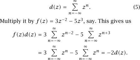
A few more examples like this will convince you that f(z)d(z) = f(l)d(z) for any polynomial function f of z and z-1. Therefore, d(z) behaves exactly like the Dirac delta δ(z - 1), at least for polynomial test functions f. Note that d(z) cannot converge for any z: the positive powers have a convergent sum only for |z| < 1, and the negative powers only for |Z| > 1. The “function” d(z) is an example of a formal power series: any series ![]() where the coefficients an can be anything and we ignore all convergence issues.
where the coefficients an can be anything and we ignore all convergence issues.
By inspection, these formal power series are “holomorphic” throughout the punctured plane: after all, holomorphic just means that the complex derivative d/dz exists, and the derivative Σn nanzn-1 of a formal power series clearly remains a formal power series. (By contrast, nonholomorphic series would involve the complex conjugate z.)
So that is what a vertex operator looks like: a formal power series ![]() , where each coefficient an is now an operator (endomorphism) on the space
, where each coefficient an is now an operator (endomorphism) on the space ![]() of states, which is an infinite-dimensional vector space. Since the vertex operators are in one-to-one correspondence with the states (we called this the “state-field correspondence” above), we can label these vertex operators with states: the standard convention is to denote the vertex operator corresponding to state v ∈
of states, which is an infinite-dimensional vector space. Since the vertex operators are in one-to-one correspondence with the states (we called this the “state-field correspondence” above), we can label these vertex operators with states: the standard convention is to denote the vertex operator corresponding to state v ∈ ![]() by
by
![]()
The symbol “Y” should remind you of the sphere with three legs, which as we know is the vertex of string theory. These coefficients vn are the modes: as in any quantum field theory, all observables and states in the theory are built up from them.
The most important state in the theory is the vacuum |0〉. It corresponds to the identity vertex operator: Y(|0〉, z) = I. From the physical point of view, the vertex operator Y(v, z) is the field that created the state v at time t = -∞ i.e., Y(v,O)|O〉 exists and equals v. (Recall that in our model z = 0 corresponds to t = -∞.) Among other things, this means that v-1(|0〉) = v, so indeed the modes applied to |0〉 generate ![]() , as is required in any quantum field theory.
, as is required in any quantum field theory.
The most important observable in the theory is the Hamiltonian, or energy operator, which we denote by L0. It is diagonalizable (so ![]() can be written as a sum of L0-eigenspaces) and all of its eigenvalues must be integers. For example, the vacuum |0〉 has 0 energy: L0|a〉 = 0. Since |0〉 should have the minimum energy, the L0-decomposition of
can be written as a sum of L0-eigenspaces) and all of its eigenvalues must be integers. For example, the vacuum |0〉 has 0 energy: L0|a〉 = 0. Since |0〉 should have the minimum energy, the L0-decomposition of ![]() is then
is then ![]() , where
, where ![]() 0 =
0 = ![]() |0〉. Each space
|0〉. Each space ![]() n turns out to be finite dimensional, and we can think of L0 as defining a
n turns out to be finite dimensional, and we can think of L0 as defining a ![]() + -grading on state space
+ -grading on state space ![]() .
.
The most important vertex operator in the theory is the stress-energy tensor T(z). The corresponding state is called the conformal vector ω: Y(ω, z) = T(z). This means that ω has modes ωn = Ln-1 that form a representation (4) of the Virasoro algebra ![]() . (This is the algebraic expression for the requirement of con-formal symmetry.) The conformal vector has energy 2: ω ∈
. (This is the algebraic expression for the requirement of con-formal symmetry.) The conformal vector has energy 2: ω ∈ ![]() 2.
2.
So far our theory is seriously underdetermined. The most important axiom to help us to pin it down further is locality. With a little work, one can show that this reduces to the condition that the commutator [Y(u, z), Y(v, w)] of two vertex operators should be a finite linear combination of the Dirac delta δ(z - w) = ![]() and its derivatives (∂K/∂wk)δ(z - w). Now, (z - w)k+1(∂k/∂wk)δ(z - w) = 0. To see this, look at the case k = 1:
and its derivatives (∂K/∂wk)δ(z - w). Now, (z - w)k+1(∂k/∂wk)δ(z - w) = 0. To see this, look at the case k = 1:

The proof for general k is similar. Therefore, locality can be recast in an equivalent form as follows: given any u, v ∈ ![]() , there is a positive number N such that
, there is a positive number N such that
![]()
This equation may look strange. Why can we not simply divide out the (z - n)N and get that all vertex operators commute? The reason is that when formal power series are involved, there can be zero divisors. For example, it is easy to check that (z - 1)Σn∈![]() zn = 0. Locality in the form (7) is at the heart of VOAs; for instance, one can express it as a triply infinite sequence of identities that the modes must obey, and this emphasizes just how restrictive a condition it is, and how correspondingly interesting it is to find examples of VOAs.
zn = 0. Locality in the form (7) is at the heart of VOAs; for instance, one can express it as a triply infinite sequence of identities that the modes must obey, and this emphasizes just how restrictive a condition it is, and how correspondingly interesting it is to find examples of VOAs.
This completes the definition of a VOA. A consequence of these properties is that the modes un respect the L0-grading that we mentioned earlier. This means that if u has energy k and v has energy l, then un (v) has energy k + l - n - 1. The definition followed here is sometimes called a VOA of CFT-type, for obvious reasons. Sometimes in the literature some of these conditions are weakened or dropped. For example, much of the theory is independent of the existence of the conformal vector ω, although to us it will be crucial, for reasons that will be explained in the next subsection.
A VOA is simultaneously a physical and a mathematical object. We have emphasized their physical origins in order to help explain the motivation for studying them. We know they should be valuable to mathematics, simply because CFT is, and indeed this is the case, as we shall see in section 4. But from a purely mathematical point of view, they might appear somewhat ad hoc, as though we had a list of mathematical ingredients and said to ourselves, “Let’s consider this, and then have some of these, oh, and perhaps one of those too, but with the following extra assumption:. . . .” Fortunately, there are more abstract formulations of VOAs that make them appear much less arbitrary as mathematical structures. For example, Huang has shown that they can be regarded as “two-dimensionalized” Lie algebras, in the following sense. If you want to keep track of the Lie brackets in an expression such as [a, [[b, c], d]] (which is important since the Lie bracket is not an associative operation), you can do so with the help of a binary tree, and in fact it is easy to formulate Lie algebras in the language of such trees. If one then replaces binary trees by diagrams made out of spheres with legs, as we did with Feynman diagrams earlier, one obtains a structure that is equivalent to a VOA. (Of course, this is very far from a full explanation of what Huang did: his proof is extremely long.)
3.2 Basic Properties
We see from the definition sketched in the last subsection that a VOA is an infinite-dimensional ![]() +-graded vector space with infinitely many products (namely u *n v = un((v)), which obey infinitely many identities. Needless to say, it is not an easy definition, and there are no easy examples.
+-graded vector space with infinitely many products (namely u *n v = un((v)), which obey infinitely many identities. Needless to say, it is not an easy definition, and there are no easy examples.
However, if we ignore the conformal symmetry (i.e., the conformal vector ω), then there are some simple, though uninteresting, examples. The easiest is the one-dimensional algebra ![]() =
= ![]() |0〉. More generally, a VOA
|0〉. More generally, a VOA ![]() that obeys (7) with N = 0 is a commutative associative algebra with a unit 1 = |0〉. It also has a derivation T = L-1, with respect to the product u * v = u-1(v): this means a linear map that obeys the product rule satisfied by derivatives, namely T(u * v) = (Tu) * v + u * (Tv). The converse of this statement is true too: any such algebra is a VOA that obeys (7) with N = 0. In these simple examples, the role of the derivation T is to recover the z-dependence of the vertex operator.
that obeys (7) with N = 0 is a commutative associative algebra with a unit 1 = |0〉. It also has a derivation T = L-1, with respect to the product u * v = u-1(v): this means a linear map that obeys the product rule satisfied by derivatives, namely T(u * v) = (Tu) * v + u * (Tv). The converse of this statement is true too: any such algebra is a VOA that obeys (7) with N = 0. In these simple examples, the role of the derivation T is to recover the z-dependence of the vertex operator.
Therefore, we need N not to be zero in (7) if we want interesting examples. Likewise, the vertex operators Y(u, z) must be distributions (that is, they must involve doubly infinite sums) or again the VOA reduces to a commutative associative algebra.
It is also easy to show that in any VOA (again the existence of the conformal vector is not needed), the space ![]() is a Lie algebra, with Lie bracket given by [uv] = u0(v). This is important because each
is a Lie algebra, with Lie bracket given by [uv] = u0(v). This is important because each ![]() n will carry a representation of this Lie algebra, and
n will carry a representation of this Lie algebra, and ![]() 1 generates continuous symmetries of the VOA (at least when
1 generates continuous symmetries of the VOA (at least when ![]() 1 ≠ {0}). For a typical VOA
1 ≠ {0}). For a typical VOA ![]() these Lie algebras are very familiar For instance, for the VOAs associated with rational CFT, they are reductive, which means that they are a direct sum of copies of the trivial Lie algebra
these Lie algebras are very familiar For instance, for the VOAs associated with rational CFT, they are reductive, which means that they are a direct sum of copies of the trivial Lie algebra ![]() with simple Lie algebras.
with simple Lie algebras.
The existence of the conformal vector becomes important when one starts to consider the representation theory of VOAs. A ![]() -module is defined in a natural way. We shall not give full details here, but, roughly speaking, it is a space on which
-module is defined in a natural way. We shall not give full details here, but, roughly speaking, it is a space on which ![]() acts in such a way that as much as possible of the VOA structure is respected. For example,
acts in such a way that as much as possible of the VOA structure is respected. For example, ![]() will automatically be a module for itself, just as a group acts on itself in a simple way. (See REPRESENTATION THEORY [IV.9 §2] for an explanation of the latter.) A rational VOA is defined to be one that has the simplest representation theory: it has only finitely many irreducible V-modules, and any
will automatically be a module for itself, just as a group acts on itself in a simple way. (See REPRESENTATION THEORY [IV.9 §2] for an explanation of the latter.) A rational VOA is defined to be one that has the simplest representation theory: it has only finitely many irreducible V-modules, and any ![]() -module is a direct sum of irreducible ones. They are called rational VOAs because they are the VOAs that come from rational CFT. For these VOAs,
-module is a direct sum of irreducible ones. They are called rational VOAs because they are the VOAs that come from rational CFT. For these VOAs, ![]() acts irreducibly on itself.
acts irreducibly on itself.
Assume now that ![]() is rational. Any irreducible
is rational. Any irreducible ![]() -module M will inherit from
-module M will inherit from ![]() an L0-grading by rational numbers, M = ⊕h Mh, into finite-dimensional spaces Mh. The character χM(τ) is defined by
an L0-grading by rational numbers, M = ⊕h Mh, into finite-dimensional spaces Mh. The character χM(τ) is defined by
![]()
where c is the central charge. This definition arises naturally in CFT as well as in Lie theory (or affine Kac–Moody algebras), although the curious “c/24,” needed for (9) below, is mysterious in Lie theory. (In CFT it has a natural explanation as a certain topological effect.) These characters converge for any τ in the upper half-plane ![]() . They carry a representation of the modular group SL2 (
. They carry a representation of the modular group SL2 (![]() ):
):
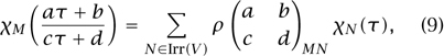
where Irr(V) denotes the (finite) set of irreducible V-modules, and ρ ![]() is a matrix with complex entries, whose rows and columns are labeled by M, N ∈ Irr(V). Equation (9) holds for any
is a matrix with complex entries, whose rows and columns are labeled by M, N ∈ Irr(V). Equation (9) holds for any ![]() in SL2 (Z), i.e., for any integers a, b, c, d satisfying ad - bc = 1. The lengthy proof of (9), by Zhu, is perhaps the high point of VOA theory, and owes much to the intuitions of rational CFT. In the next section, we shall get some idea of why it is so important.
in SL2 (Z), i.e., for any integers a, b, c, d satisfying ad - bc = 1. The lengthy proof of (9), by Zhu, is perhaps the high point of VOA theory, and owes much to the intuitions of rational CFT. In the next section, we shall get some idea of why it is so important.
4 What Are VOAs Good For?
This section describes what are probably the two most significant applications of VOAs. But let us begin by listing (without any explanations) a few others. Inspired by the geometry of string theory, vertex operator (super)algebras have been assigned to manifolds, resulting in a powerful, though complicated, algebraic invariant of those manifolds that generalizes and enriches more classical data such as de Rham cohomology. VOAs associated with affine Kac–Moody algebras at “degenerate” levels k are deeply related to the geometric Langlands program. The modularity of affine algebra characters, as well as that of, for example, lattice theta functions, are all special cases of Zhu’s theorem, which places these modularities in a much broader context.
4.1 The Mathematical Formulation of CFT
Since the 1970s quantum field theory has had considerable success, especially in geometry, by studying classical structures using infinite-dimensional methods; this is a theme in particular of Atiyah’s school. Conformal field theories are a class of exceptionally symmetric quantum field theories, and they are also among the simplest nontrivial quantum field theories known. In the past two decades mathematics has feasted on this combination of symmetry and (relative) simplicity, often by “looping” or “complexifying” more classical structures, and the impact of CFT (or, equivalently, of string theory) has been especially significant and broad. In hindsight the importance of CFT to mathematics is not surprising: it is a coherent and intricate structure that straddles several disparate areas of mathematics, sprawling across geometry, number theory, analysis, combinatorics, and indeed algebra.
From this point of view, a crucial application of VOA theory has been to CFT itself. Quantum field theories are notoriously difficult to put on a rigorous mathematical footing. But the successful applications suggest that these difficulties are a symptom of mathematical profundity and subtlety rather than of irreparable mathematical incoherence. In this sense the situation is highly reminiscent of the deep conceptual challenges to eighteenth-century mathematicians that were raised by calculus. The definition of a VOA by Richard Borcherds makes the chiral algebra of a CFT completely rigorous, as well as concepts like the operator product expansion. Subsequent work (especially by Huang and Zhu) reconstructs from the VOA more and more of the CFT, in arbitrary genus. The resulting clarity makes the whole subject more accessible to, and hence exploitable by, mathematicians. Quantum field theories are here to stay in mathematics, and thanks to VOAs mathematicians are absorbing a large class of them completely and explicitly.
4.2 Monstrous Moonshine
In 1978 McKay noticed that 196884 ≈ 196883. Why was this an interesting observation? Well, the number on the left is the first meaningful coefficient of the j-FUNCTION [IV.1 8]

the generator of all modular functions for SL2 (96). Recall that a modular function is a function f (τ) that is meromorphic in the upper half-plane ![]() and invariant under the usual action of SL2 (
and invariant under the usual action of SL2 (![]() ). It should also be meromorphic at the boundary points
). It should also be meromorphic at the boundary points ![]() ∪ {i∞}, which are called cusps; we did not mention this condition earlier. The j-function generates these functions in the sense that any such modular function f(τ) can be written as a rational function poly(j(τ))/poly(j(τ)). In other words, j(τ) is a uniformizing function that identifies (
∪ {i∞}, which are called cusps; we did not mention this condition earlier. The j-function generates these functions in the sense that any such modular function f(τ) can be written as a rational function poly(j(τ))/poly(j(τ)). In other words, j(τ) is a uniformizing function that identifies (![]() ∪
∪ ![]() ∪ {i∞})/SL2(
∪ {i∞})/SL2(![]() ) with the Riemann sphere
) with the Riemann sphere ![]() ∪ ∞. We bracketed the constant term 744 in (10) because although 744 was the traditional choice it can be freely replaced with any other number, including 0.
∪ ∞. We bracketed the constant term 744 in (10) because although 744 was the traditional choice it can be freely replaced with any other number, including 0.
The number on the right in McKay’s observation is the dimension of the smallest nontrivial representation of the Monster, the most exceptional of the FINITE SIMPLE GROUPS [V.7]. This relation between modular functions and the Monster was completely unexpected, as they seem to occupy completely independent spots in the mathematical universe. Conway, Norton, and others fleshed out and expanded McKay’s original observation by making a number of conjectures, collectively called Monstrous Moonshine. For instance, with every pair (g, h) of commuting elements in the Monster (a group of size about 8 × 1053), we expect there to be associated a function j(g,h)(τ) that generates all modular functions for some discrete subgroup Γ(g,h) of SL2 (![]() ). The j-function would be assigned in the case g = h = identity.
). The j-function would be assigned in the case g = h = identity.
The first major step toward proving these Moonshine conjectures was made by Frenkel, Lepowsky, and Meur-man in the mid 1980s. They constructed an infinite- dimensional vector space V![]() out of formal power series. They were motivated on the one hand by the vertex operators of string theory, and on the other by the formally similar distributions used in constructing affine algebra representations. This seemed a promising direction since for both string theory and affine algebra representations modular functions arise naturally. Together with a rich algebraic structure that came from these “vertex operators,” V
out of formal power series. They were motivated on the one hand by the vertex operators of string theory, and on the other by the formally similar distributions used in constructing affine algebra representations. This seemed a promising direction since for both string theory and affine algebra representations modular functions arise naturally. Together with a rich algebraic structure that came from these “vertex operators,” V![]() was also acted on in a natural way by the Monster group. Moreover, although V
was also acted on in a natural way by the Monster group. Moreover, although V![]() is infinite dimensional, it comes packaged into finite-dimensional pieces
is infinite dimensional, it comes packaged into finite-dimensional pieces ![]() , and the “graded dimension” Σn, dim(
, and the “graded dimension” Σn, dim(![]() )qn equals j - 744. The action of the Monster sends each
)qn equals j - 744. The action of the Monster sends each ![]() to itself; that is, each space
to itself; that is, each space ![]() itself carries a representation of the Monster. Frenkel, Lepowsky, and Meurman proposed that V
itself carries a representation of the Monster. Frenkel, Lepowsky, and Meurman proposed that V![]() lies at the heart of the Monstrous Moonshine conjectures.
lies at the heart of the Monstrous Moonshine conjectures.
Borcherds was struck by the formal similarity between V![]() and the chiral algebras of CFTs, and by abstracting out their important algebraic properties he defined a new structure called a vertex (operator) algebra. His axioms clarified their relationship with (generalizations of) Kac–Moody algebras, and by 1992 he had proved the main Conway–Norton conjecture (which corresponds to the case where g is arbitrary but h is the identity in the conjecture given earlier). Although his definition of VOAs required a deep understanding of the physics of CFT, his elaborate proof of this Moonshine conjecture is purely algebraic.
and the chiral algebras of CFTs, and by abstracting out their important algebraic properties he defined a new structure called a vertex (operator) algebra. His axioms clarified their relationship with (generalizations of) Kac–Moody algebras, and by 1992 he had proved the main Conway–Norton conjecture (which corresponds to the case where g is arbitrary but h is the identity in the conjecture given earlier). Although his definition of VOAs required a deep understanding of the physics of CFT, his elaborate proof of this Moonshine conjecture is purely algebraic.
We would now call V![]() a rational VOA with only one irreducible module (namely itself); its symmetry group is the Monster and its character (8) is j(τ) - 744. The removal of the constant term 744 from (10) is significant as it says that the Lie algebra
a rational VOA with only one irreducible module (namely itself); its symmetry group is the Monster and its character (8) is j(τ) - 744. The removal of the constant term 744 from (10) is significant as it says that the Lie algebra ![]() is trivial—this is necessary if the symmetry group is to be finite. It is conjectured that V
is trivial—this is necessary if the symmetry group is to be finite. It is conjectured that V![]() is the unique VOA with central charge c = 24, trivial
is the unique VOA with central charge c = 24, trivial ![]() 1 and only one irreducible module. This is meant to be reminiscent of the LEECH LATTICE [I.4 §4], which is known to be the unique twenty-four-dimensional even self-dual lattice with no vectors of length
1 and only one irreducible module. This is meant to be reminiscent of the LEECH LATTICE [I.4 §4], which is known to be the unique twenty-four-dimensional even self-dual lattice with no vectors of length ![]() . Indeed, the Leech lattice plays a crucial role in the construction of V
. Indeed, the Leech lattice plays a crucial role in the construction of V![]() .
.
Most of the Moonshine conjectures are still open and this deep connection between modular functions and the Monster is still somewhat mysterious. At the time of writing, however, VOAs still provide the only serious approach to the Moonshine conjectures.
Borcherds defined VOAs to clarify the chiral algebra of CFT and to tackle Monstrous Moonshine. For this work, he was awarded a Fields Medal in 1998.
Further Reading
Borcherds, R. E. 1986. Vertex algebras, Kac–Moody algebras, and the Monster. Proceedings of the National Academy of Sciences of the USA 83:3068-71.
——. 1992. Monstrous Moonshine and monstrous Lie superalgebras. Inventiones Mathematicae 109:405–44.
Di Francesco, P., P. Mathieu, and D. Sénéchal. 1996. Conformal Field Theory. New York: Springer.
Gannon, T. 2006. Moonshine Beyond the Monster: The Bridge Connecting Algebra, Modular Forms and Physics. Cambridge: Cambridge University Press.
Kac, V. G. 1998. Vertex Algebras for Beginners, 2nd edn. Providence, RI: American Mathematical Society.
Lepowsky, J., and H. Li. 2004. Introduction to Vertex Operator Algebras and their Representations. Boston, MA: Birkhäuser.
1. More precisely, for quantum fields, locality takes the form that if not even light can connect two given space-rime points, then the quantum fields at those points must be causally independent. In particular, measurements at such points can be performed simultaneously with arbitrary precision. In quantum theories, this requires those operators to commute. Equation (2) is a generous way to satisfy locality.