---

IV.15 Operator Algebras

Nigel Higson and John Roe

---

1 The Beginnings of Operator Theory

We can ask two basic questions about any equation, or system of equations: is there a solution, and, if there is, is it unique? Experience with finite systems of linear equations indicates that the two questions are interconnected. Consider for instance the equations

2x + 3y - 5z = a,

x - 2y + z = b,

3x +y - 4z = c.

Notice that the left-hand side of the third equation is the sum of the left-hand sides of the first two. As a result, no solution to the system exists unless a + b = c. But if a + b = c, then any solution of the first two equations is also a solution of the third; and in any linear system involving more unknowns than equations, solutions, when they exist, are never unique. In the present case, if (x, y, z) is a solution, then so is (x + t, y + t, z + t), for any t. Thus the same phenomenon (a linear relation among the equations) that prevents the system from admitting solutions in some cases also prevents solutions from being unique in other cases.

To make the relation between existence and uniqueness of solutions more precise, consider a general system of linear equations of the form

k₁₁u₁ + k₁₂u₂ + · · · + k_1nu_n = f₁,

k₂₁u₁ + k₂₂u₂ + · · · + k_2nu_n = f₂,

.         
.         
.         

k_n1u₁ + k_n2u₂ + · · · + k_nnu_n = f_n

consisting of n equations in n unknowns. The scalars k_ji form a matrix of coefficients and the problem is to solve for the u_i in terms of the f_j. The general theorem illustrated by our particular numerical example above is that the number of linear conditions that the f_j must satisfy if a solution is to exist is equal to the number of arbitrary constants appearing in the general solution when a solution does exist. To use a more technical vocabulary, the dimension of the KERNEL [I.3 §4.1] of the matrix K = {k_ji} is equal to the dimension of its cokernel. In the example, these numbers are both 1.

A little more than a hundred years ago, FREDHOLM [VI.66] made a study of integral equations of the type

u(y) - ∫ k(y, x)u(x) dx = f (y)

These arose from questions in theoretical physics, and the problem was to solve for the function u in terms of the function f. Since an integral can be thought of as a limit of finite sums, Fredholm’s equation is an infinite-dimensional counterpart of the finite-dimensional linear systems considered above, in which vectors with n components are replaced by functions with values at infinitely many different points x. (Strictly speaking, Fredholm’s equation is analogous to a matrix equation of the type u - Ku = f rather than Ku = f. The altered form of the left-hand side has no effect on the overall behavior of the matrix equation, but it does considerably alter the behavior of the integral equation. As we shall see, Fredholm was fortunate to work with a class of equations whose behavior mirrors that of matrix equations very closely.)

A very simple example is

u(y) - u(x) dx = f(y).

To solve this equation, it helps to observe that the quantity u (x) dx, when thought of as a function of y, is a constant. Thus in the homogeneous case (f ≡ 0), the only possible solutions for u(y) are the constant functions. On the other hand, for a general function f, solutions exist if and only if the single linear condition f(y) dy = 0 is satisfied. So in this example the dimension of the kernel and the dimension of the cokernel are both 1. Fredholm set out on a systematic exploration of the analogy between matrix theory and integral equations that this example suggests. He was able to prove that, for equations of his type, the dimensions of the kernel and of the cokernel are always finite and equal.

Fredholm’s work sparked the imagination of HILBERT [VI.63], who made a detailed study of the integral operators that transform u(y) into ∫ k(y, x)u(x) dx, in the special case where the real-valued function k is symmetric, meaning that k(x, y) = k(y, x). The finite-dimensional counterpart of Hilbert’s theory is the theory of real symmetric matrices. Now if K is such a matrix, then a standard result from linear algebra asserts that there is an orthonormal basis consisting of EIGENVECTORS [I.3 §4.3] for K, or equivalently that there is a unitary matrix U such that U^-1TU is diagonal. (Unitary means that U is invertible and preserves the lengths of vectors: ||Uv|| = ||v|| for all vectors v.) Hilbert obtained an analogous theory for all symmetric integral operators. He showed that there exist functions u₁ (y), u₂(y), . . . and real numbers λ_l, λ₂, . . . such that

∫ k(y, x)u_n (x) dx = λ_n u_n(y)

Thus u_n(y) is an eigenfunction for the integral operator, with eigenvalue λ_n.

In most cases it is hard to calculate u_n and λ_n explicitly, but calculation is possible when k(x, y) = ϕ(x - y) for some periodic function ϕ. If the range of integration is [0, 1] and the period of ϕ is 1, then the eigenfunctions are cos(2kπy), k = 0, 1, 2, . . . , and sin(2kπy), k = 1, 2, . . . . In this case, the theory of FOURIER SERIES [III.27] tells us that a general function f (y) on [0, 1] can be expanded as the sum of a series Σ(ak cos 2kπy + b_k sin 2kπy) of cosines and sines. Hilbert showed that, in general, there is an analogous expansion

f(y) = Σa_nu_n(y)

in terms of the eigenfunctions for any symmetric integral operator. In other words, the eigenfunctions form a basis, just as in the finite-dimensional case. Hilbert’s result is now called the spectral theorem for symmetric integral operators.

1.1 From Integral Equations to Functional Analysis

Hilbert’s spectral theorem led to an explosion of activity, since integral operators arise in many different areas of mathematics (including, for example, the DIRICHLET PROBLEM [IV.12 §1] in partial differential equations and the REPRESENTATION THEORY OF COMPACT GROUPS [IV.9 §3]). It was soon recognized that these operators are best viewed as linear transformations on the HILBERT SPACE [III.3 7] of all functions u(y) such that ∫ |u(y)|² dy < ∞. Such functions are called square-integrable, and the collection of all of them is denoted L² [0, 1].

With the important concept of Hilbert space available, it became convenient to examine a much broader range of operators than the integral operators initially considered by Fredholm and Hilbert. Since Hilbert spaces are VECTOR SPACES [I.3 §2.3] and METRIC SPACES [III.56], it made sense to look first at operators from a Hilbert space to itself that are both linear and continuous: these are usually called bounded linear operators. The analogue of the symmetry condition k(x, y) = k(y, x) on integral operators is the condition that a bounded linear operator T be self-adjoint, which is to say that (Tu, v) = (u, Tv) for all vectors u and v in the Hilbert space (the angle brackets denote the inner product). A simple example of a self-adjoint operator is the multiplication operator by a real-valued function m(y); this is the operator M defined by the formula (Mu)(y) = m(y)u(y). (The finite-dimensional counterpart to a multiplication operator is a diagonal matrix K, which multiplies the jth component of the vector by the matrix entry k_jj.)

Hilbert’s spectral theorem for symmetric integral operators tells us that every such operator can be given a particularly nice form: with respect to a suitable “basis” of L² [0,1], namely a basis of eigenfunctions, it will have an infinite diagonal matrix. Moreover, the basis vectors can be chosen to be orthogonal to each other. For a general self-adjoint operator, this is not true. Consider, for instance, the multiplication operator from L² [0, 1] to itself that takes each square-integrable function u(y) to the function yu(y). This operator has no EIGENVECTORS [I.3 §4.3], since if λ is an EIGEN- VALUE [I.3 §4.3], then we need yu(y) = λu(y) for every y, which implies that u(y) = 0 for every y not equal to λ, and hence that ∫ |u(y)|² dy = 0. However, this example is not particularly worrying, since a multiplication operator of this kind is a sort of continuous analogue of the operator defined by a diagonal matrix. It turns out that if we enlarge our concept of “diagonal” to include multiplication operators, then all self-adjoint operators are “diagonalizable,” in the sense that, after a suitable “change of basis,” they become multiplication operators.

To make this statement precise, we need the notion of the SPECTRUM [III.86] of an operator T. This is the set of complex numbers λ for which the operator T - λI does not have a bounded inverse (here I is the identity operator on Hilbert space). In finite dimensions the spectrum is precisely the set of eigenvalues, but in infinite dimensions this is not always so. Indeed, whereas every symmetric matrix has at least one eigenvalue, a self-adjoint operator, as we have just seen, need not. As a result of this, the spectral theorem for bounded self-adjoint operators is phrased not in terms of eigenvalues but in terms of the spectrum. One way of formulating it is to state that any self-adjoint operator T is unitarily equivalent to a multiplication operator (Mu)(y) = m(y)u(y), where the closure of the range of the function m(y) is the spectrum of T. Just as in the finite-dimensional case, a unitary operator is an invertible operator U that preserves the lengths of vectors. To say that T and M are unitarily equivalent is to say that there is some unitary map U, which we can think of as an analogue of a change-of-basis matrix, such that T = U^-1MU. This generalizes the statement that any real symmetric matrix is unitarily equivalent to a diagonal matrix with the eigenvalues along the diagonal.

1.2 The Mean Ergodic Theorem

A beautiful application of the spectral theorem was found by VON NEUMANN [VI.91]. Imagine a checkerboard on which are distributed a certain number of checkers. Imagine that for each square there is designated a “successor” square (in such a way that no two squares have the same successor), and that every minute the checkers are rearranged by moving each one to its successor square. Now focus attention on a single square and each minute record with a 1 or 0 whether or not there is a piece on the square. This produces a succession of readings R₁, R₂, R₃, . . . like this:

00100110010110100100 · · ·.

We might expect that over time, the average number of positive readings R_J = 1 will converge to the number of pieces on the board divided by the number of squares. If the rearrangement rule is not complicated enough, then this will not happen. For example, in the most extreme case, if the rule designates each square

as its own successor, then the readout will be either 00000 · · · or 111111 · · ·, depending on whether or not we chose a square with a piece on it to begin with. But if the rule is sufficiently complicated, then the “time average” (1/n) will indeed converge to the number of pieces on the board divided by the number of squares, as expected.

The checkerboard example is elementary, since in fact the only “sufficiently complicated” rules in this finite case are cyclic permutations of the squares of the board, and thus all the squares move past our observation post in succession. However, there are related examples where one observes only a small fraction of the data. For instance, replace the set of squares on a checkerboard with the set of points on a circle, and in place of the checkers, imagine that a subset S of a circle is marked as occupied. Let the rearrangement rule be the rotation of points on the circle through some irrational number of degrees. Stationed at a point x of the circle, we record whether x belongs to S, the first rotated copy of S, the second rotated copy of S, and so on to obtain a sequence of 0 or 1 readings as before. One can show that (for nearly every x) the time average of our observations will converge to the proportion of the circle occupied by S.

Similar questions about the relationship between time and space averages had arisen in thermodynamics and elsewhere, and the expectation that time and space averages should agree when the rearrangement rule is sufficiently complex became known as the ergodic hypothesis.

Von Neumann brought operator theory to bear on this question in the following way. Let H be the Hilbert space of functions on the squares of the checkerboard, or the Hilbert space of square-integrable functions on the circle. The rearrangement rule gives rise to a unitary operator U on H by means of the formula

(Uf)(y) = f(ϕ^-1(y)),

where ϕ is the function describing the rearrangement. Von Neumann’s ergodic theorem asserts that if no non-constant function in H is fixed by U(this is one way of saying that the rearrangement rule is “sufficiently complicated”), then, for every function f ∈ H, the limit

exists and is equal to the constant function whose value everywhere is the average value of f. (To apply this to our examples, take f(x) to be the function that is 1 if the point x is occupied and 0 otherwise.)

Von Neumann’s theorem can be deduced from a spectral theorem for unitary operators that is analogous to the spectral theorem for self-adjoint operators. Every unitary operator can be reduced to a multiplication operator, not by real-valued functions but by functions whose values are complex numbers of absolute value 1. The key to the proof then becomes a statement about complex numbers of absolute value 1: if z is such a complex number, different from 1, then the expression (1/n) approaches zero as n →, ∞. This in turn is easily proved using the formula for the sum of a geometric series, = z(1 - z_n) / (1 - z). (More detail can be found in ERGODIC THEOREMS [V.9].)

1.3 Operators and Quantum Theory

Von Neumann realized that Hilbert spaces and their operators provide the correct mathematical tools to formalize the laws of quantum mechanics, introduced in the 1920s by Heisenberg and Schrödinger.

The state of a physical system at any given instant is the list of all the information needed to determine its future behavior. If, for instance, the system consists of a finite number of particles, then classically its state consists of the list of the position and momentum vectors of all the constituent particles. By contrast, in von Neumann’s formulation of quantum mechanics one associates with each physical system a Hilbert space H, and a state of the system is represented by a unit vector u in H. (If u and v are unit vectors and v is a scalar multiple of u, then u and v determine the same state.)

Associated with each observable quantity (perhaps the total energy of the system, or the momentum of one particle within the system) is a self-adjoint operator Q on H whose spectrum is the set of all observed values of that quantity (hence the origin of the term “spectrum”). States and observables are related as follows: when a system is in the state described by a unit vector u ∈ H, the expected value of the observable quantity corresponding to a given self-adjoint operator Q is the inner product 〈Qu, u〉. This may not be a value that is ever actually measured: rather, it is the average of values that are obtained from many repeated experiments with the system when it is in the given state u. The relation between states and observables reflects the paradoxical behavior of quantum mechanics: it is possible, and in fact typical, for a system to exist in a “superposed” state, under which repeated identical experiments produce distinct outcomes. A measurement of an observable quantity will produce a determinate outcome if and only if the state of the system is an eigenvector for the operator associated with that quantity.

A distinctive feature of quantum theory is that the operators associated with different observables typically do not commute with one another. If two operators do not commute, then they will typically have no eigenvectors in common, and, as a result, simultaneous measurements of two different observables will typically not result in determinate values for both of them. A famous example is provided by the operators P and Q associated with the position and momentum of a particle moving along a line. They satisfy the Heisenberg commutation relation

QP - PQ = ,

where is a certain physical constant. (This is an instance of a general principle which relates the noncommutativity of observables in quantum mechanics to the Poisson bracket of the corresponding observables in classical mechanics: see MIRROR SYMMETRY [IV.16 §§2.1.3, 2.2.1].) As a result, it is impossible for the particle simultaneously to have a determinate momentum and position. This is the uncertainty principle.

It turns out that there is an essentially unique way of representing the Heisenberg commutation relation using self-adjoint operators on Hilbert space: the Hilbert space H must be L² (); the operator P must be and the operator Q must be multiplication by x. This theorem allows one to determine explicitly the observable operators for simple physical systems. For example, in a system consisting of a particle on a line subject to a force directed toward the origin which is proportional to the distance from the origin (as if the particle were attached to a spring, anchored at the origin), the operator for total energy is

where k is a constant which determines the overall strength of the force. The spectrum of this operator is the set

{(n + )(k/m)^1/2 : n = 0, 1, 2, . . .}.

These are therefore the possible values for the total energy of the system. Notice that the energy can assume only a discrete set of values. This is another characteristic and fundamental feature of quantum theory.

Another important example is the operator of total energy for the hydrogen atom. Like the operator above, this may be realized as a certain explicit partial differential operator. It can be shown that the eigenvalues of this operator form a sequence proportional to { -1, -, , . . .}. A hydrogen atom, when disturbed, may release a photon, resulting in a drop in its total energy. The released photon will have energy equal to the difference between the energies of the initial and final states of the atom, and therefore it is proportional to a number of the form 1/n² - 1/m². When light from hydrogen is passed through a prism or diffraction grating, bright lines are indeed observed at wavelengths corresponding to these possible energies. Spectral observations of this sort provide experimental confirmation for quantum mechanical predictions.

So far we have discussed states of a quantum system only at a single instant. However, quantum systems evolve in time, just as classical systems do: to describe this evolution we need a law of motion. The time evolution of a quantum system is represented by a family of unitary operators U_t : H →. H, parametrized by the real numbers. If the system is in an initial state u, it will be in the state U_tu after t units of time. Because the passage of s units of time followed by t further units is the same as the passage of s + t units, the unitary operators U_t satisfy the group law U_sU_t = U_{s + t}. An important theorem of Marshall Stone asserts that there is a one-to-one correspondence between unitary groups {U_t} and self-adjoint operators E given by the formula

The quantum law of motion is that the generator E corresponding in this way to time evolution is the operator associated with the observable “total energy.” When E is realized as a differential operator on a Hilbert space of functions (as in the examples above), this statement becomes a differential equation, the Schrödinger equation.

1.4 The GNS Construction

The time-evolution operators U_t of quantum mechanics satisfy the law U_sU_t = U_{s + t}. More generally, we define a unitary representation of a GROUP [I.3 §2.1] G to be a family of unitary operators U_g, one for each g ∈ G, satisfying the law U_g1g2 = U_g1U_g2 for all g_l, g₂ ∈ G. Originally introduced by FROBENIUS [VI.58] as a tool for the study of finite groups, REPRESENTATION THEORY [IV.9] has become indispensable in mathematics and physics wherever the symmetries of a system must be taken into account.

If U is a unitary representation of G and v is a vector, then σ : g 〈U_g v, v〉 is a function defined on G. The law U_g1g2 = U_g1, U_g2 implies that σ has an important positivity property, namely

for any scalars a_g ∈ . A function defined on G and having this positivity property is said to be positive definite. Conversely, from a positive-definite function one can build a unitary representation. This GNS construction (in honor of Israel Gelfand, Mark Naimark, and Irving Segal) begins by considering the group elements themselves as basis vectors in an abstract vector space. We can attempt to define an inner product on this vector space by means of the formula

〈91,92〉 = σ( g₂).

The resulting object may differ from a genuine Hilbert space in two respects. First, there may be nonzero vectors whose length, as measured by the inner product, is zero (although the hypothesis that σ is positive definite does rule out the possibility that there might be vectors of negative length). Second, the COMPLETENESS AXIOM [III.62] of Hilbert space theory may not be satisfied. However, there is a “completion” procedure which fixes both these deficiencies. Applied in the present case, it produces a Hilbert space H_σ that carries a unitary representation of G.

Versions of the GNS construction arise in several areas of mathematics. They have the advantage that the functions on which the constructions are based are easy to manipulate. For instance, convex combinations of positive-definite functions are again positive definite, and this allows geometrical methods to be applied to the study of representations.

1.5 Determinants and Traces

The original works of Fredholm and Hilbert borrowed heavily from traditional concepts of linear algebra, and in particular the theory of DETERMINANTS [III.15]. In view of the complicated definition of the determinant even for finite matrices, it is perhaps not surprising that the infinite-dimensional situation presented extraordinary challenges. Very soon, much simpler alternative approaches were found that avoided determinants altogether. But it is interesting to note that the determinant, or to be more exact the related notion of the trace, has played an important role in recent developments on which we will report later in this article.

The trace of an n × n matrix is the sum of its diagonal entries. As with the determinant, the trace of a matrix A is equal to the trace of BAB^-1 for any invertible matrix B. In fact, the trace is related to the determinant by the formula det(exp(A)) = exp(tr(A)) (because of the invariance properties of trace and determinant, it is enough to check this for diagonal matrices, where it is easy). In infinite dimensions the trace need not make sense since the sum of the diagonal entries of an ∞ × ∞ matrix may not converge. (The trace of the identity operator is a case in point: the diagonal entries are all 1, and if there are infinitely many of them, then their sum is not well-defined.) One way to address this problem is to limit oneself to operators for which the sum is well-defined. An operator T is said to be of trace class if, for every two sequences {u_j} and {v_j} of pairwise orthogonal vectors of length 1, the sum is absolutely convergent. A trace-class operator T has a well-defined and finite trace, namely the sum (which is independent of the choice of orthonormal basis {u_j}).

Integral operators such as those appearing in Fredholm’s equation provide natural examples of trace-class operators. If k(y, x) is a smooth function, then the operator Tu(y) = ∫ k(y, x)u(x) dx is of trace class, and its trace is equal to ∫ k(x, x) dx, which can be regarded as the “sum” of the diagonal elements of the “continuous matrix” k.

2 Von Neumann Algebras

The commutant of a set S of bounded linear operators on a Hilbert space H is the collection S′ of all operators on H that commute with every operator in the set S. The commutant of any set is an algebra of operators on H. That is, if T₁ and T₂ are in the commutant, then so are T₁ T₂ and any linear combination a₁T₁ + a₂T₂.

As mentioned in the previous section, a unitary representation of a group G on a Hilbert space U_g is a collection of unitary operators U_g, labeled by elements of G, with the property that for any two group elements g₁ and g₂ the composition U_g1 U_g2 is equal to U_g1g2. A von Neumann algebra is any algebra of operators on a complex Hilbert space H which is the commutant of some unitary representation of a group on H. Every von Neumann algebra is closed under adjoints and under limits of nearly every sort. For example, it is closed under pointwise limits: if {T_n} is a sequence of operators in a von Neumann algebra M, and if T_nv → Tv, for every vector v ∈ H, then T ∈ M.

It is easy to check that every von Neumann algebra M is equal to its own double commutant M″ (the commutant of the commutant of M). Von Neumann proved that if a self-adjoint algebra M of operators is closed under pointwise limits, then M is equal to the commutant of the group of unitary operators in its commutant, and is therefore a von Neumann algebra.

2.1 Decomposing Representations

Let g → U_g be a unitary representation of a group G on a Hilbert space H. If a closed subspace H₀ of H is mapped into itself by all the operators U_g, then it is said to be an invariant subspace for the representation. If H₀ is invariant, then since the operators U_g map H₀ to itself, their restrictions to H₀ constitute another representation of G, called a subrepresentation of the original.

A subspace H₀ is invariant for a representation, and so determines a subrepresentation, if and only if the orthogonal projection operator P : H → H₀ belongs to the commutant of that representation. This points to a close connection between subrepresentations and von Neumann algebras. In fact, von Neumann algebra theory can be thought of as the study of the ways in which unitary representations can be decomposed into subrepresentations.

A representation is irreducible if it has no nontrivial invariant subspace. A representation that does have a nontrivial invariant subspace H₀ can be divided into two subrepresentations: those associated with H₀ and those associated with its orthogonal complement . Unless both the representations H₀ and are irreducible, we will be able to divide one or both of them into still smaller pieces by repeating the process that was just carried out for H. If the initial Hilbert space H is finite dimensional, then continuing in this way we will eventually decompose it into irreducible subrepresentations. In the language of matrices, we will obtain a basis for H with respect to which all the operators in the group are simultaneously block diagonal, in such a way that each block represents an irreducible group of unitary operators on a smaller Hilbert space.

Reducing a unitary representation on a finite-dimensional Hilbert space into irreducible subrepresentations is a bit like decomposing an integer into a product of prime factors. As with prime factorization, the decomposition process for a finite-dimensional unitary representation has only one possible end: there is, up to ordering, a unique list of irreducible representations into which a given unitary representation decomposes. But in infinite dimensions the decomposition process faces a number of difficulties, the most surprising of which is that there may be two decompositions of the same representation into entirely different sets of irreducible subrepresentations.

In the face of this, a different form of decomposition suggests itself, which is roughly analogous to the factorization of an integer into prime powers instead of individual primes. Let us refer to the prime powers into which an integer is decomposed as its components. They have two characteristic properties: no two components share a common factor, and any two (proper) factors of the same component do share a common factor. Similarly, one can decompose a unitary representation into isotypical components, which have analogous properties: no two distinct isotypical components share a common (meaning isomorphic) subrepresentation, and any two subrepresentations of the same isotypical component have themselves a common subsubrepresentation. Any unitary representation (finite dimensional or not) can be decomposed into isotypical components, and this decomposition is unique.

In finite dimensions, every isotypical representation decomposes into a (finite) number of identical irreducible subrepresentations (like the prime factors of a prime power). In infinite dimensions this is not so. In effect, much of von Neumann algebra theory is concerned with analyzing the many possibilities that arise.

2.2 Factors

The commutant of an isotypical unitary representation is called a factor. Concretely, a factor is a von Neumann algebra M whose center, the set of all operators in M that commute with every member of M, consists of nothing more than scalar multiples of the identity operator. This is because projections in the center of M correspond to projections onto combinations of isotypical subrepresentations. Every von Neumann algebra can be uniquely decomposed into factors.

A factor is said to be of type I if it arises as the commutant of an isotypical representation that is a multiple of a single irreducible representation. Every type I factor is isomorphic to the algebra of all bounded operators on a Hilbert space. In finite dimensions, every factor is of type I, since as we already noted every isotypical representation decomposes into a multiple of one irreducible representation.

The existence of unitary representations with more than one decomposition into irreducible components is related to the existence of factors that are not of type I. Von Neumann, together with Francis Murray, investigated this possibility in a series of papers that mark the foundation of operator algebra theory. They introduced an order structure on the collection of subrepresentations of a given isotypical representation or, to put it in terms of the commutant, on the collection of projections in a given factor. If H₀ and H₁ are subrepresentations of the isotypical representation H, then we write H₀ H₁ if H₀ is isomorphic to a subrepresentation of H₁. Murray and von Neumann proved that this is a total ordering: either H₀ H₁; or H₁ H₀; or both, in which case H₀ and H₁ are isomorphic. For example, in a finite-dimensional type I situation, where H is a multiple of n copies of a single irreducible representation, each subrepresentation is the sum of m ≤ n copies of the irreducible representation, and the order structure of the (isomorphism classes of) subrepresentations is the same as the order structure of the integers {0, 1, . . . , n}.

Murray and von Neumann showed that the only order structures that can arise from factors are the following very simple ones:

Type I,     {0, 1, 2, . . . , n} or {0, 1, 2, . . . , ∞}

Type II,    [0, 1] or [0, ∞];

Type III,  {0, ∞}.

The type of a factor is determined from the order structure of its projections according to this table.

In the case of factors of type II, the order structure is that of an interval of real numbers, not integers. Any subrepresentation of an isotypical representation of type II can be divided into yet smaller subrepresentations: we shall never reach an irreducible “atom.” Nevertheless, subrepresentations can still be compared in size by means of the “real-valued dimension” provided by Murray and von Neumann’s theorem.

A notable example of a factor of type II may be obtained as follows. Let G be a group and let H = l² (G) be a Hilbert space having basis vectors [g] corresponding to the elements g ∈ G. Then there is a natural representation of G on H derived from the group multiplication law, called the regular representation: given an element g of G, the corresponding unitary map U_g is the linear operator that takes each basis vector [g′] in l² (G) to the basis vector [gg′]. The commutant of this representation is a von Neumann algebra M. If G is a commutative group, then all the operators U_g are in the center of M; but if G is far enough from commutativity (for instance, if it is a free group), then M will have trivial center and will therefore be a factor. It can be shown that this factor is of type II. There is a simple explicit formula for the real-valued dimension of a subrepresentation corresponding to an orthogonal projection P ∈ M. Represent P by an infinite matrix relative to the basis {[g]} of H. Because P commutes with the representation, it is easy to see that the diagonal elements of P are all the same, equal to some real number between 0 and 1. This real number is the dimension of the subrepresentation corresponding to P.

More recently, the Murray-von Neumann dimension theory has found unexpected applications in TOPOLOGY [I.3 §6.4]. Many important topological concepts, such as Betti numbers, are defined as the (integer-valued) dimensions of certain vector spaces. Using von Neumann algebras, one can define real-valued counterparts of these quantities that have useful additional properties. In this way, one can use von Neumann algebra theory to obtain topological conclusions. The von Neumann algebras used here are typically obtained by the construction of the previous paragraph from the FUNDAMENTAL GROUP [IV.6 §2] of some compact space.

2.3 Modular Theory

Type III factors remained rather mysterious for a long time; indeed, Murray and von Neumann were at first unable to determine whether any such factors existed. They eventually managed to do so, but the fundamental breakthrough in the area came well after their pioneering work, when it was realized that each von Neumann algebra has a special family of symmetries, its so-called modular automorphism group.

To explain the origins of modular theory, let us consider once again the von Neumann algebra obtained from the regular representation of a group G. We defined the operators U_g on l² (G) by multiplying on the left by elements of G; but we could equally well have considered a representation defined by multiplying on the right. This would have yielded a different von Neumann algebra.

So long as we deal only with discrete groups G this difference is unimportant, because the map S : [g] → [g^-1] is a unitary operator on H that interchanges the left and right regular representations. But for certain continuous groups the problem arises that the function f (g) may be square-integrable while f (g^-1) is not. In this situation there is no simple unitary isomorphism analogous to the one for discrete groups. To remedy this, one must introduce a correction factor called the modular function of G.

The project of modular theory is to show that something analogous to the modular function can be constructed for any von Neumann algebra. This object then serves as an invariant for all factors of type III, whether or not they are explicitly derived from groups.

Modular theory exploits a version of the GNS construction (section 1.4). Let M be a self-adjoint algebra of operators. A linear functional φ : M → is called a state if it is positive in the sense that φ(T*T) ≥ 0, for every T ∈ M (this terminology is derived from the connection described earlier between Hilbert space theory and quantum mechanics). For the purposes of modular theory we restrict attention to faithful states, those for which φ (T*T) = 0 implies T = 0. If φ is a state, then the formula

〈T₁, T₂〉 = φ(T₁ * T₂)

defines an inner product on the vector space M. Applying the GNS procedure, we obtain a Hilbert space H_M. The first important fact about H_M is that every operator T in M determines an operator on H_M. Indeed, a vector V ∈ H_M is a limit V = lim_n→∞ V_n of elements in M, and we can apply an operator T ∈ M to the vector V using the formula

where on the right-hand side we use multiplication in the algebra M. Because of this observation, we can think of M as an algebra of operators on H_M, rather than as an algebra of operators on whatever Hilbert space we began with.

Next, the adjoint operation equips the Hilbert space H_M with a natural “antilinear” operator S : H_M → H_M by the formula¹ S(V) = V*. Since for the regular representation, this is indeed analogous to the operator S we encountered in our discussion of continuous groups. The important theorem of Minoru Tomita and Masamichi Takesaki asserts that, as long as the original state ϕ satisfies a continuity condition, the complex powers U_t = (S * S)^it have the property that U_tMU_-t = M, for all t.

The transformations of M given by the formula T U_tTU_-t are called the modular automorphisms of M. Alain Connes proved that they depend only in a rather inessential way on the original faithful state ϕ. To be precise, changing ϕ changes the modular automorphisms only by inner automorphisms, that is, transformations of the form T UTU^-1, where U is a unitary operator in M itself. The remarkable conclusion is that every von Neumann algebra M has a canonical oneparameter group of “outer automorphisms,” which is determined by M alone and not by the state ϕ that is used to define it.

The modular group of a type I or type II factor consists only of the identity transformation; however, the modular group of a type III factor is much more complex. For example, the set

{t ∈ : T U_tTU_-t is an inner automorphism}

is a subgroup of and an invariant of M that can be used to distinguish between uncountably many different type III factors.

2.4 Classification

A crowning achievement of von Neumann algebra theory is the classification of factors that are approximately finite dimensional. These are the factors that are in a certain sense limits of finite-dimensional algebras. Besides the range of the dimension function, which separates factors into types, the sole invariant is the module. This is a flow on a certain space that is assembled from the modular automorphism group.

A lot of attention is currently being given to the longstanding problem of distinguishing among the type II factors associated with the regular representations of groups. Of special interest is the case of FREE GROUPS [Iν.10 §2], around which has flourished the subject of free probability theory. Despite intensive effort, some fundamental questions remain open: at the time of writing it is unknown whether the factors associated with the free groups on two and on three generators are isomorphic.

Another important development has been subfactor theory, which attempts to classify the ways in which factors can be realized within other factors. A remarkable and surprising theorem of Vaughan Jones shows that, in the type II situation, where continuous values of dimensions are the norm, the dimensions of subfactors can in certain situations assume only a discrete range of values. The combinatorics associated with this result have also appeared in other apparently quite unrelated parts of mathematics, notably KNOT THEORY [III.44].

3 C*-Algebras

Von Neumann algebra theory helps describe the structure of a single representation of a group on a Hilbert space. But in many situations it is of interest to gain an understanding of all possible unitary representations. To shed some light on this problem we turn to a related but different part of operator algebra theory.

Consider the collection B(H) of all bounded operators on a Hilbert space H. It has two very different structures: algebraic operations, such as addition, multiplication, and formation of adjoints; and analytic structures, such as the operator norm

||T|| = sup{||Tu|| : ||u|| ≤ 1}.

These structures are not independent of one another. Suppose, for instance, that ||T|| < 1 (an analytic hypothesis). Then the geometric series

S = I + T + T² + T₃ + · · ·

converges in B(H), and its limit S satisfies

S(I - T) = (I - T)S = I.

It follows that I - T is invertible in B(H) (an algebraic conclusion). One can easily deduce from this that the spectral radius r(T) of any operator T (defined to be the greatest absolute value of any complex number in the spectrum of T) is less than or equal to its norm.

The remarkable spectral radius formula goes much further in the same direction. It asserts that r(T) lim_n∞||Tⁿ||^1/n If T is normal (TT* = T*T), and in particular if T is self-adjoint, then it may be shown that ||T|| = ||T||ⁿ. As a result, the spectral radius of T is precisely equal to the norm of T. There is therefore a very close connection between the algebraic structure of (H), particularly algebraic structure related to the adjoint operation, and the analytic structure.

Not all the properties of (H) are relevant to this connection between algebra and analysis. A C*-algebra A is an abstract structure that has enough properties for the argument of the previous two paragraphs to remain valid. A detailed definition would be out of place here, but it is worth mentioning that a crucial condition relating norm, multiplication, and *-operation is

||a*a|| = ||a||², a ∈ A,

called the C*-identity for A. We also note that special classes of operators on Hilbert space (unitaries, orthogonal projections, and so on) all have their counterparts in a general C*-algebra. For example, a unitary u ∈ A satisfies uu* = u*u = 1, and a projection p satisfies p = p² = p*.

A simple example of a C*-algebra is obtained by starting with a single operator T ∈ (H). The collection of all operators S ∈ (H) that can be obtained as limits of polynomials in T and T* is a C*-algebra said to be generated by T. The C*-algebra generated by T is commutative if and only if T is normal; this is one reason for the importance of normal operators.

3.1 Commutative C*-Algebras

If X is a COMPACT [III.9] TOPOLOGICAL SPACE [III.90], then the collection C(X) of continuous functions f : X - comes with natural algebraic operations (inherited from the usual ones on ) and a norm ||f|| = sup {|f(x)| : x ∈ X}. In fact, these operations make C(X) into a C*- algebra. The multiplication in C(X) is commutative, because the multiplication of complex numbers is commutative.

A basic result of Gelfand and Naimark asserts that every commutative C*- algebra is isomorphic to some C(X). Given a commutative C*- algebra A, one constructs X as the collection of all algebra homomorphisms ξ : A → , and the Gelfand transform then associates with a ∈ A the function ξ ξ(a) from X to .

The Gelfand–Naimark theorem is a foundational result of operator theory. For example, a modern proof of the spectral theorem might proceed as follows. Let T be a self-adjoint or normal operator on a Hilbert space H, and let A be the commutative C*- algebra generated by T. By the Gelfand–Naimark theorem, A is isomorphic to C(X) for some space X, which may in fact be identified with the spectrum of T. If v is a unit vector in H, then the formula S 〈Sv, v〉 defines a state ϕ on A. The GNS space associated with this state is a Hilbert space of functions on X, and elements of A = C(X) act as multiplication operators. In particular, T acts as a multiplication operator. A small additional argument shows that T is unitarily equivalent to this multiplication operator, or at least to a direct sum of such operators (which is itself a multiplication operator on a larger space).

Continuous functions can be composed: if f and g are continuous functions (with the range of g contained in the domain of f), then f ο g is also a continuous function. Since the Gelfand–Naimark theorem tells us that any self-adjoint element of a C* -algebra A sits inside an algebra isomorphic to the continuous functions on the spectrum of a, we conclude that if a ∈ A is self-adjoint, and if f is a continuous function defined on the spectrum of a, then an operator f (a) exists in A. This functional calculus is a key technical tool in C*-algebra theory. For example, suppose that u ∈ A is unitary and ||u - 1|| < 2. Then the spectrum of u is a subset of the unit circle in that does not contain -1. One can define a continuous branch of the complex logarithm function on such a subset, and it follows that there is an element a = log u of the algebra such that a = -a* and u = e^a. The path t e^ta, 0 ≤ t ≤ 1, is then a continuous path of unitaries in A connecting u to the identity. Thus every unitary sufficiently close to the identity is connected to the identity by a unitary path.

3.2 Further Examples of C*-Algebras

3.2.1 The Compact Operators

An operator on a Hilbert space has finite rank if its range is a finite-dimensional subspace. The operators of finite rank form an algebra, and its closure is a C*-algebra called called the algebra of compact operators and denoted . One can also view as a “limit” of matrix algebras

M₁() → M₂() → M₃() → · · ·,

where each matrix algebra is included in the next by

Many natural operators are compact, including the integral operators that arose in Fredholm’s theory. The identity operator on a Hilbert space is compact if and only if that Hilbert space is finite dimensional.

3.2.2 The CAR Algebra

The presentation of as a limit of matrix algebras leads one to consider other “limits” of a similar sort. (We shall not attempt a formal definition of these limits here, but it is important to note that the limit of a sequence A₁ → A₂ → A₃ → · · · depends on the homomorphisms A_i → A_i+1 as well as on the algebras A_i.) One particularly important example is obtained as the limit

M₁ () → M₂() → M₄() → · · ·,

where each matrix algebra is included in the next by

This is called the CAR algebra, because it contains elements that represent the canonical anticommutation relations that arise in quantum theory. C*-algebras find several applications to quantum field theory and quantum statistical mechanics which extend von Neumann’s formulation of quantum theory in terms of Hilbert space.

3.2.3 Group C*-Algebras

If G is a group and g U_g is a unitary representation of G on a Hilbert space H, we can consider the smallest C*-algebra of operators on H containing all the U_g; this is called the C* -algebra generated by the representation. An important example is the regular representation on the Hilbert space l²(G) generated by G, which we defined in section 2.2. The C*-algebra that it generates is denoted (G). The subscript “r” refers to the regular representation. Considering other representations leads to other, potentially different, group C*-algebras.

Consider, for example, the case G = . Since this is a commutative group, its C*-algebra is also commutative, and thus it is isomorphic to C(X) for a suitable X, by the Gelfand–Naimark theorem. In fact, X is the unit circle S₁, and the isomorphism

takes a function on the circle to its Fourier series.

States defined on group C*-algebras correspond to positive-definite functions defined on groups, and hence to unitary group representations. In this way new representations may be constructed and studied. For example, using states of group C*-algebras it is possible to give to the set of irreducible representations of G the structure of a topological space.

3.2.4 The Irrational Rotation Algebra

The algebra C*() is generated by a single unitary element U (corresponding to 1 ∈ ). Moreover, it is the universal example of such a C*-algebra, which is to say that given any C*-algebra A and unitary u ∈ A there is one and only one homomorphism C* () → A sending U to u. In fact, this is nothing other than the functional calculus homomorphism for the unitary u.

If instead we consider the universal example of a C*-algebra generated generated by two unitaries U, V subject to the relation

UV = e^2παVU,

where α is irrational, we obtain a noncommutative C*-algebra called the irrational rotation algebra Aα. The irrational rotation algebras have been studied intensively from a number of points of view. Using K-theory (see below) it has been shown that A_α1 is isomorphic to A_α2 if and only if α₁ ± α₂ is an integer.

It can be shown that the irrational rotation algebra is simple, which implies that any pair of unitaries U, V satisfying the commutation relation above will generate a copy of A_α. (Note the contrast with the case of a single unitary: 1 is a unitary operator, but it does not generate a copy of C* ().) This allows us to give a concrete representation of A_α on the Hilbert space L² (S¹), where U is the rotation through 2πα and V is multiplication by z : S¹ → .

4 Fredholm Operators

A Fredholm operator between Hilbert spaces is defined to be a bounded operator T for which the kernel and cokernel are finite dimensional. This means that the homogeneous equation Tu = 0 admits only finitely many linearly independent solutions, while the inhomogeneous equation Tu = v admits a solution if v satisfies a finite number of linear conditions. The terminology arises from Fredholm’s original work on integral equations; he showed that if K is an integral operator, then I + K is a Fredholm operator.

For the operators that Fredholm considered, the dimensions of the kernel and cokernel must be equal, but in general this need not be so. The unilateral shift operator S, which maps the infinite “row vector” (a₁, a₂, a₃,. . .) to (0, a₁, a₂,. . .), is an example. The equation Su = 0 has only the zero solution, but the equation Su = v has a solution only if the first coordinate of the vector v is zero.

The index of a Fredholm operator is defined to be the integer difference

index(T) = dim(ker(T)) - dim(coker(T)).

For example, every invertible operator is a Fredholm operator of index 0, whereas the unilateral shift is a Fredholm operator of index -1.

4.1 Atkinson’s Theorem

Consider the two systems of linear equations

Although the coefficients of these equations are very close, the dimensions of their kernels are quite different: the left-hand system has only the zero solution, whereas the right-hand system has the nontrivial solutions (t, -2t). Thus the dimension of the kernel is an unstable invariant of the system of equations. A similar remark applies to the dimension of the cokernel. By contrast, the index is stable, despite its definition as the difference of two unstable quantities.

An important theorem of Frederick Atkinson gives precise expression to these stability properties. Atkinson’s theorem asserts that an operator T is Fredholm if and only if it is invertible modulo compact operators. This implies that any operator that is sufficiently close to a Fredholm operator is itself a Fredholm operator with the same index, and that if T is a Fredholm operator and K is a compact operator, then T + K is a Fredholm operator with the same index as T. Notice that, since integral operators are compact operators, this contains Fredholm’s original theorem as a special case.

4.2 The Toeplitz Index Theorem

TOPOLOGY [I.3 §6.4] studies those properties of mathematical systems that remain the same when the system is (continuously) perturbed. Atkinson’s theorem tells us that the Fredholm index is a topological quantity. In many contexts it is possible to obtain a formula for the index of a Fredholm operator in terms of other, apparently quite different, topological quantities. Formulas of this sort often indicate deep connections between analysis and topology and often have powerful applications.

The simplest example involves the Toeplitz operators. A Toeplitz operator has a matrix with the special form

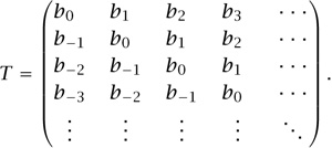
In other words, as you go down each diagonal of the matrix, the entries remain constant. The sequence of coefficients defines defines a function f(z) = on the unit circle in the complex plane, called the symbol of the Toeplitz operator. It can be shown that a Toeplitz operator whose symbol is a continuous function which is never zero is Fredholm. What is its index?

The answer is given by thinking about the symbol as a mapping from the unit circle to the nonzero complex numbers: in other words, as a closed path in the nonzero complex plane. The fundamental topological invariant of such a path is its winding number: the number of times it “goes around” the origin in the counterclockwise direction. It can be proved that the index of a Toeplitz operator with nonzero symbol f is minus the winding number of f. For example, if f is the function f(z) = z (with winding number +1), then the associated Toeplitz operator is the unilateral shift S that we encountered earlier (with index -1). The Toeplitz index theorem is a very special case of THE ATIYAH-SINGER INDEX THEOREM [V.2], which gives a topological formula for the indices of various Fredholm operators that arise in geometry.

4.3 Essentially Normal Operators

Atkinson’s theorem suggests that compact perturbations of an operator are in some sense “small.” This leads to the study of properties of an operator that are preserved by compact perturbation. For instance, the essential spectrum of an operator T is the set of complex numbers λ for which T - λI fails to be Fredholm (that is, invertible modulo compact operators). Two operators T₁ and T₂ are essentially equivalent if there is a unitary operator U such that UT₁ U* and T₂ differ by a compact operator. A beautiful theorem originally due to WEYL [VI.80] asserts that two self-adjoint or normal operators are essentially equivalent if and only if they have the same essential spectrum.

One might argue that the restriction to normal operators in this theorem is inappropriate. Since we are concerned with properties that are preserved by compact perturbation, would it not be more appropriate to consider essentially normal operators—that is, operators T for which T*T - TT* is compact? This apparently modest variation leads to an unexpected result. The unilateral shift S is an example of an essentially normal operator. Its essential spectrum is the unit circle, as is the essential spectrum of its adjoint; however, S and S* cannot be essentially equivalent, because S has index -1 and S* has index +1. Thus some new ingredient, beyond the essential spectrum, is needed to classify essentially normal operators. In fact, it follows easily from Atkinson’s theorem that if essentially normal operators T₁ and T₂ are to be essentially equivalent, then not only must they have the same essential spectrum but also, for every λ not in the essential spectrum, the Fredholm index of T₂ - λI must be equal to the Fredholm index of T₂ - λI. The converse of this statement was proved by Larry Brown, Ron Douglas, and Peter Fillmore in the 1970s, using entirely novel techniques that led to a new era of interaction between C*-algebra theory and topology.

4.4 K-Theory

A remarkable feature of the Brown-Douglas-Fillmore work was the appearance within it of tools from ALGEBRAIC TOPOLOGY [IV.6], notably K-theory. Remem ber that, according to the Gelfand–Naimark theorem, the study of (suitable) topological spaces and the study of commutative C*-algebras are one and the same; all the techniques of topology can be transferred, via the Gelfand–Naimark isomorphism, to commutative C*-algebras. Having made this observation, it is natural to ask which of these techniques can be extended further, to provide information about a11 C*-algebras, commutative or not. The first and best example is K-theory.

In its most basic form, K-theory associates with each C*- algebra A an Abelian group K(A), and with each homomorphism of C*-algebras a corresponding homomorphism of Abelian groups. The building blocks for K(A) can be thought of as generalized Fredholm operators associated with A; the generalization is that these operators act on “Hilbert spaces” in which the complex scalars are replaced by elements of the C*-algebra A. The group K(A) itself is defined to be the collection of connected components of the space of all such generalized Fredholm operators. Thus if A = , for instance (so that we are dealing with classical Fredholm operators), then K (A) = . This follows from the fact that two Fredholm operators are connected by a path of Fredholm operators if and only if they have the same index.

One of the great strengths of K-theory is that one can construct K-theory classes from a variety of different ingredients. For example, every projection p ∈ A defines a class in K(A) which can be thought of as a “dimension” for the range of p. This connects K-theory to the classification of factors (section 2.2), and has become an important tool in the effort to classify various families of C*-algebras, such as the irrational rotation algebras. (It was at one time thought that the irrational rotation algebras might not contain any nontrivial projections at all: the construction of such projections by Marc Rieffel was an important step in the development of C*-algebra K-theory.) Another beautiful example is George Elliott’s classification theorem for locally finite-dimensional C*-algebras like the CAR algebra; they are completely determined by K-theoretic invariants.

The problem of computing the K-theory groups of noncommutative C*- algebras, particularly group C*-algebras, has turned out to have important connections with topology. In fact, some key advances in topology have come from C*-algebra theory in this way, thereby allowing operator algebraists to repay some of the debt they owe to the topologists for K-theory. The principal organizing problem in this area is the Baum-Cornnes conjecture, which proposes a description of the K-theory of group C*-algebras in terms of invariants familiar in algebraic topology. Most of the progress on the conjecture to date is the result of work of Gennadi Kasparov, who dramatically broadened the original discoveries of Brown, Douglas, and Fillmore to cover not just single essentially normal operators but also noncommuting systems of operators, that is, C*-algebras. Kasparov’s work is now a central component of operator algebra theory.

5 Noncommutative Geometry

DESCARTES’s [VI.11] invention of coordinates showed that one can do geometry by thinking about coordinate functions rather than directly thinking about points in space and their interrelationships: these coordinate functions are the familiar x, y, and z. The Gelfand–Naimark theorem can be viewed as one expression of this idea of passing from the “point picture” of a space X to the “field picture” of the algebra C(X) of functions on it. The success of K-theory in operator algebras invites us to ponder whether the field picture might be more powerful than the point picture, since K-theory can be applied to noncommutative C*-algebras which may not have any “points” (homomorphisms to ) at all.

One of the most exciting research frontiers in operator algebra theory is reached along a path which develops these thoughts. The noncommutative geometry program of Connes takes seriously the idea that a general C*-algebra should be thought of as an algebra of functions on a “noncommutative space,” and goes on to develop “noncommutative” versions of many ideas from geometry and topology, as well as completely new constructions that have no commutative counterpart. Noncommutative geometry begins with the creative reformulation of ideas from ordinary geometry in ways that involve only operators and functions, but not points.

Consider, for instance, the circle S¹. The algebra C(S¹) reflects all the topological properties of S¹, but to incorporate its metric (distance-related) properties as well we look not just at C(S¹) but at the pair consisting of the algebra C(S¹) and the operator D = id/dθ on the Hilbert space H = L²(S¹). Notice that if f is a function on the circle (considered as a multiplication operator on H), then the commutator Df - fD is also a multiplication operator, this time by idf/dθ. It follows that ordinary measurements of angular distance between points on the circle can be recovered from C(S¹) and D by the formula

d(p, q) = max{|f(p) - f(a)| : ||Df - fD|| ≤ 1}.

Connes argues that operator |D|^-1 plays the role of the “unit of arc-length ds” in this and many other, more complicated situations.²

Another feature of the examples Connes considers, also of central importance in noncommutative geometry, is the fact that the operator |D|^-k is a trace-class operator (see section 1.5) when k is large enough. In the case of the circle, k needs to be bigger than 1. Computations with traces connect noncommutative geometry to COHOMOLOGY THEORY [IV.6 §4]. We now have two kinds of “noncommutative algebraic topology,” namely K-theory and a new variant of homology called cyclic cohomology; the connection between the two is provided by a very general index theorem.

There are several procedures that produce noncommutative C*-algebras (to which Connes’s methods can be applied) from classical geometric data. The irrational rotation algebras A_θ are examples; the classical picture to which they apply is the QUOTIENT SPACE [I.3 §3.3] of the circle by the group of rotations through multiples of θ. Classical methods of geometry and topology are unable to handle this quotient space, but the noncommutative approach via A_θ is much more successful.

An exciting but speculative possibility is that the basic laws of physics should be addressed from the perspective of noncommutative geometry. The transition to noncommutative C*-algebras can be viewed as analogous to the transition from classical to quantum mechanics. However, Connes has argued that noncommutative C*-algebras play a role in describing the physical world even before the transition is made to quantum physics.

Further Reading

Connes, A. 1995. Noncommutative Geometry. Boston, MA: Academic Press.

Davidson, K. 1996. C*-Algebras by Example. Providence, RI: American Mathematical Society.

Fillmore, P. 1996. A User’s Guide to Operator Algebras. Canadian Mathematical Society Series of Monographs and Advanced Texts. New York: John Wiley.

Halmos, P. R. 1963. What does the spectral theorem say? American Mathematical Monthly 70:241–47.

 

1. The interpretation of this formula on the completion H_M of M is a delicate matter.

2. The operator D is not quite invertible since it vanishes on constant functions. A small modification must therefore be made before considering inverse operators. The operator |D| is by definition the positive square root of D².