
IV.12 Partial Differential Equations
Sergiu Klainerman
Introduction
Partial differential equations (or PDEs) are an important class of functional equations: they are equations, or systems of equations, in which the unknowns are functions of more than one variable. As a very crude analogy, PDEs are to functions as polynomial equations (such as x2 + y2 = 1, for example) are to numbers. The distinguishing feature of PDEs, as opposed to more general functional equations, is that they involve not only unknown functions, but also various partial derivatives of those functions, in algebraic combination with each other and with other, fixed, functions. Other important kinds of functional equations are integral equations, which involve various integrals of the unknown functions, and ordinary differential equations (ODEs), in which the unknown functions depend on only one independent variable (such as a time variable t) and the equation involves only ordinary derivatives d/dt, d2/dt2, d3/dt3,. . . of these functions.
Given the immense scope of the subject the best I can hope to do is to give a very crude perspective on some of the main issues and an even cruder idea of the multitude of current research directions. The difficulty one faces in trying to describe the subject of PDEs starts with its very definition. Is it a unified area of mathematics, devoted to the study of a clearly defined set of objects (in the way that algebraic geometry studies solutions of polynomial equations or topology studies manifolds, for example), or is it rather a collection of separate fields, such as general relativity, several complex variables, or hydrodynamics, each one vast in its own right and centered on a particular, very difficult, equation or class of equations? I will attempt to argue below that, even though there are fundamental difficulties in formulating a general theory of PDEs, one can nevertheless find a remarkable unity between various branches of mathematics and physics that are centered on individual PDEs or classes of PDEs. In particular, certain ideas and methods in PDEs have turned out to be extraordinarily effective across the boundaries of these separate fields. It is thus no surprise that the most successful book ever written about PDEs did not mention PDEs in its title: it was Methods of Mathematical Physics by COURANT [VI.83] and HILBERT [VI.63].
As it is impossible to do full justice to such a huge subject in such limited space I have been forced to leave out many topics and relevant details; in particular, I have said very little about the fundamental issue of breakdown of solutions, and there is no discussion of the main open problems in PDEs. A longer and more detailed version of the article, which includes these topics, can be found at
http://press.princeton.edu/titles/8350.html
1 Basic Definitions and Examples
The simplest example of a PDE is the LAPLACE EQUATION [I.3 §5.4]
![]()
Here, Δ is the Laplacian, that is, the differential operator that transforms functions u = u(xl, x2, x3) defined from ![]() 3 to
3 to ![]() according to the rule
according to the rule
![]()
where ∂1, ∂2, ∂3 are standard shorthand for the partial derivatives ∂/∂x1, ∂/∂x2, ∂/∂x3. (We will use this shorthand throughout the article.) Two other fundamental examples (also described in [I.3 §5.4]) are the heat equation and the wave equation:

In each case one is asked to find a function u that satisfies the corresponding equations. For the Laplace equation u will depend on x1, x2, and x3, and for the other two it will depend on t as well. Observe that equations (2) and (3) again involve the symbol Δ, but also partial derivatives with respect to the time variable t. The constants k (which is positive) and c are fixed and represent the rate of diffusion and the speed of light, respectively. However, from a mathematical point of view they are not important, since if u(t, x1, x2, x3) is a solution of (3), for example, then υ(t, x1, x2, x3) = u(t, x1/c, x2/c, x3/c) satisfies the same equation with c = 1. Thus, when one is studying the equations one can set these constants to be 1. Both equations are called evolution equations because they are supposed to describe the change of a particular physical object as the time parameter t varies. Observe that (1) can be interpreted as a particular case of both (2) and (3): if u = u(t, x1, x2, x3) is a solution of either (2) or (3) that is independent of t, then ∂t u = 0, so u must satisfy (1).
In all three examples mentioned above, we tacitly assume that the solutions we are looking for are sufficiently differentiable for the equations to make sense. As we shall see later, one of the important developments in the theory of PDEs was the study of more refined notions of solutions, such as DISTRIBUTIONS [III.18], which require only weak versions of differentiability.
Here are some further examples of important PDFs. The first is THE SCHRÖDINGER EQUATION [III.83],
![]()
where u is a function from ![]() ×
× ![]() 3 to
3 to ![]() . This equation describes the quantum evolution of a massive particle, k =
. This equation describes the quantum evolution of a massive particle, k = ![]() /2m, where
/2m, where ![]() > 0 is Planck’s constant and m is the mass of the particle. As with the heat equation, one can set k to equal 1 after a simple change of variables. Though the equation is formally very similar to the heat equation, it has very different qualitative behavior. This illustrates an important general point about PDEs: that small changes in the form of an equation can lead to very different properties of solutions.
> 0 is Planck’s constant and m is the mass of the particle. As with the heat equation, one can set k to equal 1 after a simple change of variables. Though the equation is formally very similar to the heat equation, it has very different qualitative behavior. This illustrates an important general point about PDEs: that small changes in the form of an equation can lead to very different properties of solutions.
A further example is the Klein-Gordon equation
![]()
This is the relativistic counterpart to the Schrödinger equation: the parameter m has the physical interpretation of mass and mc2 has the physical interpretation of rest energy (reflecting Einstein’s famous equation E = mc2). One can normalize the constants c and mc2/![]() so that they both equal 1 by applying a suitable change of variables to time and space.
so that they both equal 1 by applying a suitable change of variables to time and space.
Though all five equations mentioned above first appeared in connection with specific physical phenomena, such as heat transfer for (2) and propagation of electromagnetic waves for (3), they have, miraculously, a range of relevance far beyond their original applications. In particular there is no reason to restrict their study to three space dimensions: it is very easy to generalize them to similar equations in n variables x1, x2, . . . ,xn.
All the PDEs listed so far obey a simple but fundamental property called the principle of superposition: if u1 and u2 are two solutions to one of these equations, then any linear combination a1u1 + a2u2 of these solutions is also a solution. In other words, the space of all solutions is a VECTOR SPACE [I.3 §2.3]. Equations that obey this property are known as homogeneous linear equations. If the space of solutions is an affine space (that is, a translate of a vector space) rather than a vector space, we say that the PDE is an inhomogeneous linear equation; a good example is Poisson’s equation:
![]()
where f : ![]() 3 →
3 → ![]() is a function that is given to us and u :
is a function that is given to us and u : ![]() 3 →
3 → ![]() is the unknown function. Equations that are neither homogeneous linear nor inhomogeneous linear are known as nonlinear. The following equation, the MINIMAL SURFACE EQUATION [III.94 §3.1], is manifestly nonlinear:
is the unknown function. Equations that are neither homogeneous linear nor inhomogeneous linear are known as nonlinear. The following equation, the MINIMAL SURFACE EQUATION [III.94 §3.1], is manifestly nonlinear:

The graphs of solutions u : ![]() 2 →
2 → ![]() of this equation are area-minimizing surfaces (like soap films).
of this equation are area-minimizing surfaces (like soap films).
Equations (1), (2), (3), (4), (5) are not just linear: they are all examples of constant-coefficient linear equations. This means that they can be expressed in the form
![]()
where ![]() is a differential operator that involves linear combinations, with constant real or complex coefficients, of mixed partial derivatives of u. (Such operators are called constant-coefficient linear differential operators.) For instance, in the case of the Laplace equation (1),
is a differential operator that involves linear combinations, with constant real or complex coefficients, of mixed partial derivatives of u. (Such operators are called constant-coefficient linear differential operators.) For instance, in the case of the Laplace equation (1), ![]() is simply the Laplacian Δ, while for the wave equation (3),
is simply the Laplacian Δ, while for the wave equation (3), ![]() is the d’Alembertian
is the d’Alembertian
![]()
The characteristic feature of linear constant-coefficient operators is translation invariance. Roughly speaking, this means that if you translate a function u, then you translate ![]() u in the same way. More precisely, if υ(x) is defined to be u(x - a) (so the value of u at x becomes the value of υ at x + a; note that x and a belong to
u in the same way. More precisely, if υ(x) is defined to be u(x - a) (so the value of u at x becomes the value of υ at x + a; note that x and a belong to ![]() 3 here), then
3 here), then ![]() υ(x) is equal to
υ(x) is equal to ![]() u(x - a). As a consequence of this basic fact we infer that solutions to the homogeneous, linear, constant-coefficient equation (8) are still solutions when translated.
u(x - a). As a consequence of this basic fact we infer that solutions to the homogeneous, linear, constant-coefficient equation (8) are still solutions when translated.
Since symmetries play such a fundamental role in PDEs we should stop for a moment to make a general definition. A symmetry of a PDE is any invertible operation T: u ![]() T(u) from functions to functions that preserves the space of solutions, in the sense that u solves the PDE if and only if T(u) solves the same PDE. A PDE with this property is then said to be invariant under the symmetry T. The symmetry T is often a linear operation, though this does not have to be the case. The composition of two symmetries is again a symmetry, as is the inverse of a symmetry, and so it is natural to view a collection of symmetries as forming a GROUP [I.3 §2.1] (which is typically a finite- or infinite-dimensional LIE GROUP [III.48 §1]).
T(u) from functions to functions that preserves the space of solutions, in the sense that u solves the PDE if and only if T(u) solves the same PDE. A PDE with this property is then said to be invariant under the symmetry T. The symmetry T is often a linear operation, though this does not have to be the case. The composition of two symmetries is again a symmetry, as is the inverse of a symmetry, and so it is natural to view a collection of symmetries as forming a GROUP [I.3 §2.1] (which is typically a finite- or infinite-dimensional LIE GROUP [III.48 §1]).
Because the translation group is intimately connected with THE FOURIER TRANSFORM [III.27] (indeed, the latter can be viewed as the representation theory of the former), this symmetry strongly suggests that Fourier analysis should be a useful tool to solve constant-coefficient PDEs, and this is indeed the case.
Our basic constant-coefficient linear operators, the Laplacian Δ and the d’Alembertian ![]() , are formally similar in many respects. The Laplacian is fundamentally associated with the geometry of EUCLIDEAN SPACE [I.3 §6.2]
, are formally similar in many respects. The Laplacian is fundamentally associated with the geometry of EUCLIDEAN SPACE [I.3 §6.2] ![]() 3 and the d’Alembertian is similarly associated with the geometry of MINKOWSKI SPACE [I.3 §6.8]
3 and the d’Alembertian is similarly associated with the geometry of MINKOWSKI SPACE [I.3 §6.8] ![]() 1+3. This means that the Laplacian commutes with all the rigid motions of the Euclidean space
1+3. This means that the Laplacian commutes with all the rigid motions of the Euclidean space ![]() 3, while the d’Alembertian commutes with the corresponding class of Poincaré transformations of Minkowski spacetime. In the former case this simply means that invariance applies to all transformations of
3, while the d’Alembertian commutes with the corresponding class of Poincaré transformations of Minkowski spacetime. In the former case this simply means that invariance applies to all transformations of ![]() 3 that preserve the Euclidean distances between points. In the case of the wave equation, the Euclidean distance has to be replaced by the space time distance between points (which would be called events in the language of relativity): if
3 that preserve the Euclidean distances between points. In the case of the wave equation, the Euclidean distance has to be replaced by the space time distance between points (which would be called events in the language of relativity): if ![]() = (t, x1, x2, x3) and Q(s, y1, y2, y3), then the distance between them is given by the formula
= (t, x1, x2, x3) and Q(s, y1, y2, y3), then the distance between them is given by the formula
dM(P, Q)2 = -(t - s)2 + (x1 - y1)2 + (x2 - y2)2 + (x3 - y3)2.
As a consequence of this basic fact we infer that all solutions to the wave equation (3) are invariant under translations and LORENTZ TRANSFORMATIONS [I.3 §6.8].
Our other evolution equations (2) and (4) are clearly invariant under rotations of the space variables x = (x1, x2, x3) ∈ ![]() 3, when t is fixed. They are also Galilean invariant, which means, in the particular case of the Schrödinger equation (4), that whenever u = u(t, x) is a solution so is the function
3, when t is fixed. They are also Galilean invariant, which means, in the particular case of the Schrödinger equation (4), that whenever u = u(t, x) is a solution so is the function ![]() for any vector υ ∈
for any vector υ ∈ ![]() 3.
3.
Poisson’s equation (6), on the other hand, is an example of a constant-coefficient inhomogeneous linear equation, which means that it takes the form
![]()
for some constant-coefficient linear differential operator ![]() and known function f. To solve such an equation requires one to understand the invertibility or otherwise of the linear operator
and known function f. To solve such an equation requires one to understand the invertibility or otherwise of the linear operator ![]() : if it is invertible then u will equal
: if it is invertible then u will equal ![]() -1 f, and if it is not invertible then either there will be no solution or there will be infinitely many solutions. Inhomogeneous equations are closely related to their homogeneous counterpart; for instance, if u1, u2 both solve the inhomogeneous equation (9) with the same inhomogeneous term f, then their difference u1 - u2 solves the corresponding homogeneous equation (8).
-1 f, and if it is not invertible then either there will be no solution or there will be infinitely many solutions. Inhomogeneous equations are closely related to their homogeneous counterpart; for instance, if u1, u2 both solve the inhomogeneous equation (9) with the same inhomogeneous term f, then their difference u1 - u2 solves the corresponding homogeneous equation (8).
Linear homogeneous PDEs satisfy the principle of superposition but they do not have to be translation invariant. For example, suppose that we modify the heat equation (2) so that the coefficient k is no longer constant but rather an arbitrary, positive, smooth function of (x1, x2, x3). Such an equation models the flow of heat in a medium in which the rate of diffusion varies from point to point. The corresponding space of solutions is not translation invariant (which is not surprising as the medium in which the heat flows is not translation invariant). Equations like this are called linear equations with variable coefficients. It is more difficult to solve them and describe their qualitative features than it is for constant-coefficient equations. (See, for example, STOCHASTIC PROCESSES [IV.24 §5.2] for an approach to equations of type (2) with variable k.) Finally, nonlinear equations such as (7) can often still be written in the form (8), but the operator ![]() is now a nonlinear differential operator. For instance, the relevant operator for (7) is given by the formula
is now a nonlinear differential operator. For instance, the relevant operator for (7) is given by the formula

where |∂u|2 = (∂1u)2 + (∂2u)2. Operators such as these are clearly not linear. However, because they are ultimately constructed from algebraic operations and partial derivatives, both of which are “local” operations, we observe the important fact that ![]() is at least still a “local” operator. More precisely, if u1 and u2 are two functions that agree on some open set D, then the expressions
is at least still a “local” operator. More precisely, if u1 and u2 are two functions that agree on some open set D, then the expressions ![]() [u1] and
[u1] and ![]() [u2] also agree on this set. In particular, if
[u2] also agree on this set. In particular, if ![]() [0] = 0 (as is the case in our example), then whenever u vanishes on a domain,
[0] = 0 (as is the case in our example), then whenever u vanishes on a domain, ![]() [u] will also vanish on that domain.
[u] will also vanish on that domain.
So far we have tacitly assumed that our equations take place in the whole of a space such as ![]() 3,
3, ![]() + ×
+ × ![]() 3, or
3, or ![]() ×
× ![]() 3. In reality one is often restricted to a fixed domain of that space. Thus, for example, equation (1) is usually studied on a bounded open domain of
3. In reality one is often restricted to a fixed domain of that space. Thus, for example, equation (1) is usually studied on a bounded open domain of ![]() 3 subject to a specified boundary condition. Here are some basic examples of boundary conditions.
3 subject to a specified boundary condition. Here are some basic examples of boundary conditions.
Example. The Dirichlet problem for Laplace’s equation on an open domain of D ⊂ ![]() 3 is the problem of finding a function u that behaves in a prescribed way on the boundary of D and obeys the Laplace equation inside.
3 is the problem of finding a function u that behaves in a prescribed way on the boundary of D and obeys the Laplace equation inside.
More precisely, one specifies a continuous function u0: ∂D → ![]() and looks for a continuous function u, defined on the closure
and looks for a continuous function u, defined on the closure ![]() of D, that is twice continuously differentiable inside D and solves the equations
of D, that is twice continuously differentiable inside D and solves the equations

A basic result in PDEs asserts that if the domain D has a sufficiently smooth boundary, then there is exactly one solution to the problem (10) for any prescribed function uo on the boundary ∂D.
Example. The Plateau problem is the problem of finding the surface of minimal total area that bounds a given curve.
When the surface is the graph of a function u on some suitably smooth domain D, in other words a set of the form {(x, y, u(x,y)) : (x,y) ∈ D}, and the bounding curve is the graph of a function u0 over the boundary ∂D of D, then this problem turns out to be equivalent to the Dirichlet problem (10), but with the linear equation (1) replaced by the nonlinear equation (7). For the above equations, it is also often natural to replace the Dirichlet boundary condition u(x) = u0(x) on the boundary ∂D with another boundary condition, such as the Neumann boundary condition n(x) · ∇xu(x) = u1(x) on ∂D, where n(x) is the outward normal (of unit length) to D at x. Generally speaking, Dirichlet boundary conditions correspond to “absorbing” or “fixed” barriers in physics, whereas Neumann boundary conditions correspond to “reflecting” or “free” barriers.
Natural boundary conditions can also be imposed for our evolution equations (2)-(4). The simplest one is to prescribe the values of u when t = 0. We can think of this more geometrically. We are prescribing the values of u at each spacetime point of form (0,x,y,z), and the set of all such points is a hyperplane in ![]() 1+3: it is an example of an initial time surface.
1+3: it is an example of an initial time surface.
Example. The Cauchy problem (or initial value problem, sometimes abbreviated to IVP) for the heat equation (2) asks for a solution u : ![]() + ×
+ × ![]() 3 →
3 → ![]() on the spacetime domain
on the spacetime domain ![]() + ×
+ × ![]() 3 = {(t,x) : t > 0, x ∈
3 = {(t,x) : t > 0, x ∈ ![]() 3}, which equals a prescribed function u0 :
3}, which equals a prescribed function u0 : ![]() 3 →
3 → ![]() on the initial time surface {0} ×
on the initial time surface {0} × ![]() 3 = ∂(
3 = ∂(![]() + ×
+ × ![]() 3).
3).
In other words, the Cauchy problem asks for a sufficiently smooth function u, defined on the closure of ![]() + ×
+ × ![]() 3 and taking values in
3 and taking values in ![]() , that satisfies the conditions
, that satisfies the conditions

The function u0 is often referred to as the initial conditions, or initial data, or just data, for the problem. Under suitable smoothness and decay conditions, one can show that this equation has exactly one solution u for each choice of data u0. Interestingly, this assertion fails if one replaces the future domain ![]() + ×
+ × ![]() 3 = {(t, x) : t > 0, x ∈
3 = {(t, x) : t > 0, x ∈ ![]() 3} by the past domain
3} by the past domain ![]() - ×
- × ![]() 3 = {(t,x) : t < 0, x ∈
3 = {(t,x) : t < 0, x ∈ ![]() 3}.
3}.
A similar formulation of the IVP holds for the Schrödinger equation (4), though in this case we can solve both to the past and to the future. However, in the case of the wave equation (3) we need to specify not just the initial position u(0, x) = u0(x) on the initial time surface t = 0, but also an initial velocity ∂tu(0, x) = u1(x), since equation (3) (unlike (2) or (4)) cannot formally determine ∂tu in terms of u. One can construct unique smooth solutions (both to the future and to the past of the initial hyperplane t = 0) to the IVP for (3) for very general smooth initial conditions u0, u1.
Many other boundary-value problems are possible. For instance, when analyzing the evolution of a wave in a bounded domain D (such as a sound wave), it is natural to work with the spacetime domain ![]() × D and prescribe both Cauchy data (on the initial boundary 0 × D) and Dirichlet or Neumann data (on the spatial boundary
× D and prescribe both Cauchy data (on the initial boundary 0 × D) and Dirichlet or Neumann data (on the spatial boundary ![]() × ∂D). On the other hand, when the physical problem under consideration is the evolution of a wave outside a bounded obstacle (for example, an electromagnetic wave), one considers instead the evolution in
× ∂D). On the other hand, when the physical problem under consideration is the evolution of a wave outside a bounded obstacle (for example, an electromagnetic wave), one considers instead the evolution in ![]() × (
× (![]() 3 D) with a boundary condition on D.
3 D) with a boundary condition on D.
The choice of boundary condition and initial conditions for a given PDE is very important. For equations of physical interest these arise naturally from the context in which they are derived. For example, in the case of a vibrating string, which is described by solutions of the one-dimensional wave equation ![]() in the domain (a,b) ×
in the domain (a,b) × ![]() , the initial conditions u = u0 and ∂tu = u1 at t = t0 amount to specifying the original position and velocity of the string. The boundary condition u(b) = u(b) = 0 is what tells us that the two ends of the string are fixed.
, the initial conditions u = u0 and ∂tu = u1 at t = t0 amount to specifying the original position and velocity of the string. The boundary condition u(b) = u(b) = 0 is what tells us that the two ends of the string are fixed.
So far we have considered just scalar equations. These are equations where there is only one unknown function u, which takes values either in the real numbers ![]() or in the complex numbers
or in the complex numbers ![]() . However, many important PDEs involve either multiple unknown scalar functions or (equivalently) functions that take values in a multidimensional vector space such as
. However, many important PDEs involve either multiple unknown scalar functions or (equivalently) functions that take values in a multidimensional vector space such as ![]() m. In such cases, we say that we have a system of PDEs. An important example of a system is that of the CAUCHY-RIEMANN EQUATIONS [I.3 §5.6]:
m. In such cases, we say that we have a system of PDEs. An important example of a system is that of the CAUCHY-RIEMANN EQUATIONS [I.3 §5.6]:
![]()
where u1, u2: ![]() 2 →
2 → ![]() are real-valued functions on the plane. It was observed by CAUCHY [VI.29] that a complex function w(x+iy) = u1(x,y)+iu2(x,y) is HOLOMORPHIC [I.3 §5.6] if and only if its real and imaginary parts u1, u2 satisfy the system (12). This system can still be represented in the form of a constant-coefficient linear PDE (8), but u is now a vector
are real-valued functions on the plane. It was observed by CAUCHY [VI.29] that a complex function w(x+iy) = u1(x,y)+iu2(x,y) is HOLOMORPHIC [I.3 §5.6] if and only if its real and imaginary parts u1, u2 satisfy the system (12). This system can still be represented in the form of a constant-coefficient linear PDE (8), but u is now a vector ![]() , and
, and ![]() is not a scalar differential operator, but rather a matrix of operators
is not a scalar differential operator, but rather a matrix of operators ![]() .
.
The system (12) contains two equations and two unknowns. This is the standard situation for a determined system. Roughly speaking, a system is called overdetermined if it contains more equations than unknowns and underdetermined if it contains fewer equations than unknowns. Underdetermined equations typically have infinitely many solutions for any given set of prescribed data; conversely, overdetermined equations tend to have no solutions at all, unless some additional compatibility conditions are imposed on the prescribed data.
Observe also that the Cauchy-Riemann operator ![]() has the following remarkable property:
has the following remarkable property:
![]()
Thus ![]() can be viewed as a square root of the two-dimensional Laplacian Δ. One can define a similar type of square root for the Laplacian in higher dimensions and, more surprisingly, even for the d’Alembertian operator
can be viewed as a square root of the two-dimensional Laplacian Δ. One can define a similar type of square root for the Laplacian in higher dimensions and, more surprisingly, even for the d’Alembertian operator ![]() in
in ![]() 1+3. To achieve this we need to have four 4 × 4 complex matrices γ1, γ2, γ3, γ4 that satisfy the property
1+3. To achieve this we need to have four 4 × 4 complex matrices γ1, γ2, γ3, γ4 that satisfy the property
γαγβ + γβγα = -2mαβI.
Here, I is the unit 4 × 4 matrix and mαβ = ![]() when α = β = 1, -
when α = β = 1, -![]() when α = β ≠ 1, and 0 otherwise. Using the γ matrices we can introduce the Dirac operator as follows. If u = (u1, u2, u3, u4) is a function in
when α = β ≠ 1, and 0 otherwise. Using the γ matrices we can introduce the Dirac operator as follows. If u = (u1, u2, u3, u4) is a function in ![]() 1+3 with values in
1+3 with values in ![]() 4, then we set Du = iγα∂αu. It is easy to check that, indeed, D2u=
4, then we set Du = iγα∂αu. It is easy to check that, indeed, D2u= ![]() u. The equation
u. The equation
![]()
is called the Dirac equation and it is associated with a free, massive, relativistic particle such as an electron.
One can extend the concept of a PDE further to cover unknowns that are not, strictly speaking, functions taking values in a vector space, but are instead sections of a VECTOR BUNDLE [IV.6 §5], or perhaps a map from one MANIFOLD [I.3 §6.9] to another; such generalized PDEs play an important role in geometry and modern physics. A fundamental example is given by the EINSTEIN FIELD EQUATIONS [IV.13]. In the simplest, “vacuum,” case, they take the form
![]()
where Ric(g) is the RICCI CURVATURE [III.78] tensor of the spacetime manifold M = (M, g). In this case the spacetime metric itself is the unknown to be solved for. One can often reduce such equations locally to more traditional PDE systems by selecting a suitable choice of coordinates, but the task of selecting a “good” choice of coordinates, and working out how different choices are compatible with each other, is a nontrivial and important one. Indeed, the task of selecting a good set of coordinates in order to solve a PDE can end up being a significant PDE problem in its own right.
PDEs are ubiquitous throughout mathematics and science. They provide the basic mathematical framework for some of the most important physical theories: elasticity, hydrodynamics, electromagnetism, general relativity, and nonrelativistic quantum mechanics, for example. The more modern relativistic quantum field theories lead, in principle, to equations in an infinite number of unknowns, which lie beyond the scope of PDEs. Yet, even in that case, the basic equations preserve the locality property of PDEs. Moreover, the starting point of a QUANTUM FIELD THEORY [IV.17 §2.1.4] is always a classical field theory, which is described by systems of PDEs. This is the case, for example, in the standard model of weak and strong interactions, which is based on the so-called Yang-Mills-Higgs field theory. If we also include the ordinary differential equations of classical mechanics, which can be viewed as one- dimensional PDEs, we see that essentially all of physics is described by differential equations. As examples of PDEs underlying some of our most basic physical theories we refer to the articles that discuss THE EULER AND NAVIER–STOKES EQUATIONS [III.23], THE HEAT EQUATION [III.36], THE SCHRÖDINGER EQUATION [III.83], and THE EINSTEIN EQUATIONS [IV.13].
An important feature of the main PDEs is their apparent universality. Thus, for example, the wave equation, first introduced by D’ALEMBERT [VI.20] to describe the motion of a vibrating string, was later found to be connected with the propagation of sound and electromagnetic waves. The heat equation, first introduced by FOURIER [VI.25] to describe heat propagation, appears in many other situations in which dissipative effects play an important role. The same can be said about the Laplace equation, the Schrödinger equation, and many other basic equations.
It is even more surprising that equations that were originally introduced to describe specific physical phenomena have played a fundamental role in several areas of mathematics that are considered to be “pure,” such as complex analysis, differential geometry, topology, and algebraic geometry. Complex analysis, for example, which studies the properties of holomorphic functions, can be regarded as the study of solutions to the Cauchy-Riemann equations (12) in a domain of ![]() 2. Hodge theory is based on studying the space of solutions to a class of linear systems of PDEs on manifolds that generalize the Cauchy-Riemann equations: it plays a fundamental role in topology and algebraic geometry. THE ATIYAH—SINGER INDEX THEOREM [V.2] is formulated in terms of a special class of linear PDEs on manifolds, related to the Euclidean version of the Dirac operator. Important geometric problems can be reduced to finding solutions to specific PDEs, typically nonlinear. We have already seen one example: the Plateau problem of finding surfaces of minimal total area that pass through a given curve. Another striking example is the UNIFORMIZATION THEOREM [V.34] in the theory of surfaces , which takes a compact Riemannian surface S (a two-dimensional surface with a RIEMANNIAN METRIC [I.3 §6.10]) and, by solving the PDE
2. Hodge theory is based on studying the space of solutions to a class of linear systems of PDEs on manifolds that generalize the Cauchy-Riemann equations: it plays a fundamental role in topology and algebraic geometry. THE ATIYAH—SINGER INDEX THEOREM [V.2] is formulated in terms of a special class of linear PDEs on manifolds, related to the Euclidean version of the Dirac operator. Important geometric problems can be reduced to finding solutions to specific PDEs, typically nonlinear. We have already seen one example: the Plateau problem of finding surfaces of minimal total area that pass through a given curve. Another striking example is the UNIFORMIZATION THEOREM [V.34] in the theory of surfaces , which takes a compact Riemannian surface S (a two-dimensional surface with a RIEMANNIAN METRIC [I.3 §6.10]) and, by solving the PDE
![]()
(which is a nonlinear variant of the Laplace equation (1)), uniformizes the metric so that it is “equally curved” at all points on the surface (or, more precisely, has constant SCALAR CURVATURE [III.78]) without changing the conformal class of the metric (i.e., without distorting any of the angles subtended by curves on the surface). This theorem is of fundamental importance to the theory of such surfaces: in particular, it allows one to give a topological classification of compact surfaces in terms of a single number χ(S), which is called the EULER CHARACTERISTIC [I.4 §2.2] Of the surface S. The three-dimensional analogue of the uniformization theorem, the GEOMETRIZATION CONJECTURE [IV.7 §2.4] Of Thurston, has recently been established by Perelman, who did so by solving yet another PDE; in this case, the equation is the RICCI FLOW [III.78] equation
![]()
which can be transformed into a nonlinear version of the heat equation (2) after a carefully chosen change of coordinates. The proof of the geometrization conjecture is a decisive step toward the total classification of all three-dimensional compact manifolds, in particular establishing the well-known POINCARÉ CONJECTURE [IV.7 §2.4]. To overcome the many technical details in establishing this conjecture, one needs to make a detailed qualitative analysis of the behavior of solutions to the Ricci flow equation, a task which requires just about all the advances made in geometric PDEs in the last hundred years.
Finally, we note that PDEs arise not only in physics and geometry but also in many fields of applied science. In engineering, for example, one often wants to control some feature of the solution u to a PDE by carefully selecting whatever components of the given data one can directly influence; consider, for instance, how a violinist controls the solution to the vibrating string equation (closely related to (3)) by modulating the force and motion of a bow on that string in order to produce a beautiful sound. The mathematical theory dealing with these types of issues is called control theory.
When dealing with complex physical systems, one cannot possibly have complete information about the state of the system at any given time. Instead, one often makes certain randomness assumptions about various factors that influence it. This leads to the very important class of equations called stochastic differential equations (SDEs), where one or more components of the equation involve a RANDOM VARIABLE [III.71 §4] of some sort. An example of this is in the BLACK-SCHOLES MODEL [VII.9 §2] in mathematical finance. A general discussion of SDEs can be found in STOCHASTIC PROCESSES [IV.24 §6].
The plan for the rest of this article is as follows. In section 2 I shall describe some of the basic notions and achievements of the general theory of PDEs. The main point I want to make here is that, in contrast with ordinary differential equations, for which a general theory is both possible and useful, partial differential equations do not lend themselves to a useful general theoretical treatment because of some important obstructions that I shall try to describe. One is thus forced to discuss special classes of equations such as elliptic, parabolic, hyperbolic, and dispersive equations. In section 3 I will try to argue that, despite the impossibility of developing a useful general theory that encompasses all, or most, of the important examples, there is nevertheless an impressive unifying body of concepts and methods for dealing with various basic equations, and this gives PDEs the feel of a well-defined area of mathematics. In section 4 I develop this further by trying to identify some common features in the derivation of the main equations that are dealt with in the subject. An additional source of unity for PDEs is the central role played by the issues of regularity and breakdown of solutions, which is discussed only briefly here. In the final section we shall discuss some of the main goals that can be identified as driving the subject.
2 General Equations
One might expect, after looking at other areas of mathematics such as algebraic geometry or topology, that there was a very general theory of PDEs that could be specialized to various specific cases. As I shall argue below, this point of view is seriously flawed and very much out of fashion. It does, however, have important merits, which I hope to illustrate in this section. I shall avoid giving formal definitions and focus instead on representative examples. The reader who wants more precise definitions can consult the online version of this article.
For simplicity we shall look mostly at determined systems of PDEs. The simplest distinction, which we have already made, is between scalar equations, such as (1)-(5), which consist of only one equation and one unknown, and systems of equations, such as (12) and (13). Another simple but important concept is that of the order of a PDE, which is defined to be the highest derivative that appears in the equation; this concept is analogous to that of the degree of a polynomial. For instance, the five basic equations (1)-(5) listed earlier are second order in space, although some (such as (2) or (4)) are only first order in time. Equations (12) and (13), as well as the Maxwell equations, are first order.1
We have seen that PDEs can be divided into linear and nonlinear equations, with the linear equations being divided further into constant-coefficient and variable- coefficient equations. One can also divide nonlinear PDEs into several further classes depending on the “strength” of the nonlinearity. At one end of the scale, a semilinear equation is one in which all the nonlinear components of the equation have strictly lower order than the linear components. For instance, equation (15) is semilinear, because the nonlinear component eu is of zero order, i.e., it contains no derivatives, whereas the linear component Δsu is of second order. These equations are close enough to being linear that they can often be effectively viewed as perturbations of a linear equation. A more strongly nonlinear class of equations is that of quasilinear equations, in which the highest- order derivatives of u appear in the equation only in a linear manner but the coefficients attached to those derivatives may depend in some nonlinear manner on lower-order derivatives. For instance, the second-order equation (7) is quasilinear, because if one uses the product rule to expand the equation, then it takes the quasilinear form

for some explicit algebraic functions F11, F12, F22 of the lower-order derivatives of u. While quasilinear equations can still sometimes be analyzed by perturbative techniques, this is generally more difficult to accomplish than it is for an analogous semilinear equation. Finally, we have fully nonlinear equations, which exhibit no linearity properties whatsoever. A typical example is the Monge-Ampère equation
det(D2u) = F(x, u, Du),
where u : ![]() u →
u → ![]() is the unknown function, Du is the GRADIENT [I.3 §5.3] of u, D2u = (∂i∂ju)1≤i,j≤n is the Hessian matrix of u, and F:
is the unknown function, Du is the GRADIENT [I.3 §5.3] of u, D2u = (∂i∂ju)1≤i,j≤n is the Hessian matrix of u, and F: ![]() n ×
n × ![]() ×
× ![]() n →
n → ![]() is a given function. This equation arises in many geometric contexts, ranging from manifold-embedding problems to the complex geometry of CALABI-YAU MANIFOLDS [III.6]. Fully nonlinear equations are among the most difficult and least well-understood of all PDEs.
is a given function. This equation arises in many geometric contexts, ranging from manifold-embedding problems to the complex geometry of CALABI-YAU MANIFOLDS [III.6]. Fully nonlinear equations are among the most difficult and least well-understood of all PDEs.
Remark. Most of the basic equations of physics, such as the Einstein equations, are quasilinear. However, fully nonlinear equations arise in the theory of characteristics of linear PDEs, which we discuss below, and also in geometry.
2.1 First-Order Scalar Equations
It turns out that first-order scalar PDEs in any number of dimensions can be reduced to systems of first- order ODEs. As a simple illustration of this important fact consider the following equation in two space dimensions:

where a1, a2, f are given real functions in the variables x = (x1, x2) ∈ ![]() 2. We associate with (17) the first-order 2 × 2 system
2. We associate with (17) the first-order 2 × 2 system

To simplify matters, let us assume that f = 0.
Suppose now that x(s) = (x1 (s), x2 (s)) is a solution of (18), and let us consider how u(x1(s), x2 (s)) varies as s varies. By the chain rule we know that
![]()
and equations (17) and (18) imply that this equals zero (by our assumption that f = 0). In other words, any solution u = u(x1, x2) of (17) with f = 0 is constant along any parametrized curve of the form x(s) = (x1 (s), x2 (s)) that satisfies (18).
Thus, in principle, if we know the solutions to (18), which are called characteristic curves for the equation (17), then we can find all solutions to (17). I say “in principle” because, in general, the nonlinear system (18) is not so easy to solve. Nevertheless, ODEs are simpler to deal with, and the fundamental theorem of ODEs, which we will discuss later in this section, allows us to solve (18) at least locally and for a small interval in s.
The fact that u is constant along characteristic curves allows us to obtain important qualitative information even when we cannot find explicit solutions. For example, suppose that the coefficients a1, a2 are smooth (or real analytic) and that the initial data is smooth (or real analytic) everywhere on the set ![]() where it is defined, except at some point x0 where it is discontinuous. Then the solution u remains smooth (or real analytic) at all points except along the characteristic curve Γ that starts at x0, or, in other words, along the solution to (18) that satisfies the initial condition x(0) = x0. That is, the discontinuity at x0 propagates precisely along Γ. We see here the simplest manifestation of an important principle, which we shall explain in more detail later: singularities of solutions to PDEs propagate along characteristics (or, more generally, hypersurfaces).
where it is defined, except at some point x0 where it is discontinuous. Then the solution u remains smooth (or real analytic) at all points except along the characteristic curve Γ that starts at x0, or, in other words, along the solution to (18) that satisfies the initial condition x(0) = x0. That is, the discontinuity at x0 propagates precisely along Γ. We see here the simplest manifestation of an important principle, which we shall explain in more detail later: singularities of solutions to PDEs propagate along characteristics (or, more generally, hypersurfaces).
One can generalize equation (17) to allow the coefficients a1, a2, and f to depend not only on x = (x1, x2) but also on u:
![]()
The associated characteristic system becomes

As a special example of (19) consider the scalar equation in two space dimensions,
![]()
which is called the Burgers equation. Here we have set a1(x,u(x)) = 1 and a2(x,u(x)) = u(x). With this choice of a1, a2, we can take x1(s) to be s in (20). Then, renaming x2(s) as x(s), we derive the characteristic equation in the form
![]()
For any given solution u of (21) and any characteristic curve (s, x(s)) we have (d/ds)u(s,x(s)) = 0. Thus, in principle, knowing the solutions to (22) should allow us to determine the solutions to (21). However, this argument seems worryingly circular, since u itself appears in (22).
To see how this difficulty can be circumvented, consider the IVP for (21): that is, look for solutions that satisfy u(0,x) = u0(x). Consider an associated characteristic curve x(s) such that, initially, x(0) = x0. Then, since u is constant along the curve, we must have u(s, x(s)) = u0(x0). Hence, going back to (22), we infer that dx/ds = u0(x0) and thus x(s) = x0+su0(x0). We thus deduce that
![]()
which implicitly gives us the form of the solution u. We see once more, from (23), that if the initial data is smooth (or real analytic) everywhere except at a point x0 of the line t = 0, then the corresponding solution is also smooth (or real analytic) everywhere in a small neighborhood V of x0, except along the characteristic curve that begins at x0. The smallness of V is necessary here because new singularities can form at large scales. Indeed, u has to be constant along the lines x + su0(x), whose slopes depend on u0(x). At a point where these lines cross we would obtain different values of u, which is impossible unless u becomes singular by this point. This blow-up phenomenon occurs for any smooth, nonconstant initial data u0.
Remark. There is an important difference between the linear equation (17) and the quasilinear equation (19). The characteristics of the first depend only on the coefficients a1 (x), a2 (x), while the characteristics of the second depend explicitly on a particular solution u of the equation. In both cases, singularities can only propagate along the characteristic curves of the equation. For nonlinear equations, however, new singularities can form at large distance scales, whatever the smoothness of the initial data.
The above procedure extends to fully nonlinear scalar equations in ![]() d such as the Hamilton-Jacobi equation
d such as the Hamilton-Jacobi equation
![]()
where u: ![]() ×
×![]() n →
n → ![]() is the unknown function, Du is the gradient of u, and the HAMILTONIAN [III.35] H :
is the unknown function, Du is the gradient of u, and the HAMILTONIAN [III.35] H : ![]() d û
d û ![]() d →
d → ![]() and the initial data u0 :
and the initial data u0 : ![]() d →
d → ![]() are given. For instance, the eikonal equation ∂tu = |Du| is a special instance of a Hamilton-Jacobi equation. We associate with (24) the ODE system
are given. For instance, the eikonal equation ∂tu = |Du| is a special instance of a Hamilton-Jacobi equation. We associate with (24) the ODE system
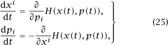
where i runs from 1 to d. The equations (25) are known as a Hamiltonian system of ODEs. The relationship between this system and the corresponding Hamilton-Jacobi equation is a little more involved than in the cases discussed above. Briefly, we can construct a solution u to (24) based only on the knowledge of the solutions (x(t), p(t)) to (25), which are called the bicharacteristic curves of the nonlinear PDE. Once again, singularities can only propagate along bicharacteristic curves (or hypersurfaces). As in the case of the Burgers equation, singularities will occur for more or less any smooth data. Thus, a classical, continuously differentiable solution can only be constructed locally in time. Both Hamilton-Jacobi equations and Hamiltonian systems play a fundamental role in classical mechanics as well as in the theory of the propagation of singularities in linear PDEs. The deep connection between Hamiltonian systems and first-order Hamilton-Jacobi equations played an important role in the introduction of the Schrödinger equation into quantum mechanics.
2.2 The Initial Value Problem for ODEs
Before we can continue with our general presentation of PDEs we need first to discuss, for the sake of comparison, the IVP for ODEs. Let us start with a first-order ODE
![]()
subject to the initial condition
![]()
Let us also assume for simplicity that (26) is a scalar equation and that f is a well-behaved function of x and u, such as f(x, u) = u3 - u + 1 + sinx. From the initial data u0 we can determine ∂xu(x0) by substituting x0 into (26). If we now differentiate the equation (26) with respect to x and apply the chain rule, we derive the equation
![]()
which for the example just defined works out to be cos x + 3u2(x)∂xu(x) - ∂xu(X). Hence,
![]()
and since ∂xu(x0) has already been determined we find that ![]() can also be explicitly calculated from the initial data u0. This calculation also involves the function f and its first partial derivatives. Taking higher derivatives of the equation (26) we can recursively determine
can also be explicitly calculated from the initial data u0. This calculation also involves the function f and its first partial derivatives. Taking higher derivatives of the equation (26) we can recursively determine ![]() as well as all other higher derivatives of u at x0. Therefore, one can in principle determine u(x) with the help of the Taylor series
as well as all other higher derivatives of u at x0. Therefore, one can in principle determine u(x) with the help of the Taylor series

We say “in principle” because there is no guarantee that the series converges. There is, however, a very important theorem, called the Cauchy-Kovalevskaya theorem, which asserts that if the function f is real analytic, as is certainly the case for our function f(x, u) = u3 - u + 1 + sinx, then there will be some neighborhood J of x0 where the Taylor series converges to a real-analytic solution u of the equation. It is then easy to show that the solution thus obtained is the unique solution to (26) that satisfies the initial condition (27). To summarize: if f is a well-behaved function, then the initial value problem for ODEs has a solution, at least in some time interval, and that solution is unique.
The same result does not always hold if we consider a more general equation of the form
![]()
Indeed, the recursive argument outlined above breaks down in the case of the scalar equation (x - x0)∂xu = f(x,u) for the simple reason that we cannot even determine ∂xu(x0) from the initial condition u(x0) = u0. A similar problem occurs for the equation (u - u0)∂Xu = f(x, u). An obvious condition that allows us to extend our previous recursive argument to (28) is to insist that a(x0, u0) ≠ 0. Otherwise, we say that the IVP (28) is characteristic. If both a and f are also real analytic, the Cauchy-Kovalevskaya theorem applies again and we obtain a unique, real-analytic solution of (28) in a small neighborhood of x0. In the case of an N × N system,
A(x, u(x))∂xu = F(x,u(x)), u(x0) = u0,
A = A(x, u) is an N × N matrix, and the noncheracteristic condition becomes
![]()
It turns out, and this is extremely important in the development of the theory of ODEs, that, while the nondegeneracy condition (29) is essential to obtain a unique solution of the equation, the analyticity condition is not at all important: it can be replaced by a simple local Lipschitz condition for A and F. It suffices to assume, for example, that their first partial derivatives exist and that they are locally bounded. This is always the case if the first derivatives of A and F are continuous.
Theorem (the fundamental theorem of ODEs). If the matrix A(x0, u0) is invertible and if A and F are continuous and have locally bounded first derivatives, then there is some time interval J ⊂ ![]() that contains x0, and a unique solution2 u defined on J that satisfies the initial conditions u(x0) = u0.
that contains x0, and a unique solution2 u defined on J that satisfies the initial conditions u(x0) = u0.
The proof of the theorem is based on the Picard iteration method. The idea is to construct a sequence of approximate solutions u(n)(x) that converge to the desired solution. Without loss of generality we can assume A to be the identity matrix.3 One starts by setting u(0)(x) = u0 and then defines, recursively,
∂xu(n) (x) = F(x, u(n-1)(x)), u(n-l) (x0) = u0.
Observe that at every stage all we need to solve is a very simple linear problem, which makes Picard iteration easy to implement numerically. As we shall see below, variations of this method are also used for solving nonlinear PDEs.
Remark. In general, the local existence theorem is sharp, in the sense that its conditions cannot be relaxed. We have seen that the invertibility condition for A(x0, u0) is necessary. Also, it is not always possible to extend the interval J in which the solution exists to the whole of the real line. As an example, consider the nonlinear equation ∂xu = u2 with initial data u = u0 at x = 0, for which the solution u = u0/(1 - xu0) becomes infinite in finite time: in the terminology of PDEs, it blows up.
In view of the fundamental theorem and the example mentioned above, one can define the main goals of the mathematical theory of ODEs as follows.
(1) Find criteria for global existence. In the case of blow-up describe the limiting behavior.
(ii) In the case of global existence describe the asymptotic behavior of solutions and families of solutions.
Though it is impossible to develop a general theory that achieves both goals (in practice one is forced to restrict oneself to special classes of equations motivated by applications), the general local existence and uniqueness theorem mentioned above provides a powerful unifying theme. It would be very helpful if a similar situation were to hold for general PDEs.
2.3 The Initial Value Problem for PDEs
In the one-dimensional situation one specifies initial conditions at a point. The natural higher-dimensional analogue is to specify them on hypersurfaces ![]() ⊂
⊂ ![]() d, that is, (d - 1)-dimensional subsets (or, to be more precise, submanifolds). For a general equation of order k, that is, one that involves k derivatives, we need to specify the values of u and of its first k - 1 derivatives in the direction normal to
d, that is, (d - 1)-dimensional subsets (or, to be more precise, submanifolds). For a general equation of order k, that is, one that involves k derivatives, we need to specify the values of u and of its first k - 1 derivatives in the direction normal to ![]() . For example, in the case of the second-order wave equation (3) and the initial hyperplane t = 0 we need to specify initial data for u and ∂tu.
. For example, in the case of the second-order wave equation (3) and the initial hyperplane t = 0 we need to specify initial data for u and ∂tu.
If we wish to use initial data of this kind to start obtaining a solution, it is important that the data should not be degenerate. (We have already seen this in the case of ODEs.) For this reason, we make the following general definition.
Definition. Suppose that we have a kth-order quasilinear system of equations, and the initial data comes in the form of the first k - 1 normal derivatives that a solution u must satisfy on a hypersurface ![]() . We say that the system is noncharacteristic at a point x0 of
. We say that the system is noncharacteristic at a point x0 of ![]() if we can use the initial data to determine formally all the other higher partial derivatives of u at x0, in terms of the data.
if we can use the initial data to determine formally all the other higher partial derivatives of u at x0, in terms of the data.
As a very rough picture to have in mind, it may be helpful to imagine an infinitesimally small neighborhood of x0. If the hypersurface ![]() is smooth, then its intersection with this neighborhood will be a piece of a (d - 1)-dimensional affine subspace. The values of u and the first k - 1 normal derivatives on this intersection are given by the initial data, and the problem of determining the other partial derivatives is a problem in linear algebra (because everything is infinitesimally small). To say that the system is noncharacteristic at x0 is to say that this linear algebra problem can be uniquely solved, which is the case provided that a certain matrix is invertible. This is the nondegeneracy condition referred to earlier.
is smooth, then its intersection with this neighborhood will be a piece of a (d - 1)-dimensional affine subspace. The values of u and the first k - 1 normal derivatives on this intersection are given by the initial data, and the problem of determining the other partial derivatives is a problem in linear algebra (because everything is infinitesimally small). To say that the system is noncharacteristic at x0 is to say that this linear algebra problem can be uniquely solved, which is the case provided that a certain matrix is invertible. This is the nondegeneracy condition referred to earlier.
To illustrate the idea, let us look at first-order equations in two space dimensions. In this case ![]() is a curve Γ, and since k - 1 = 0 we must specify the restriction of u to Γ ⊂
is a curve Γ, and since k - 1 = 0 we must specify the restriction of u to Γ ⊂ ![]() 2 but we do not have to worry about any derivatives. Thus, we are trying to solve the system
2 but we do not have to worry about any derivatives. Thus, we are trying to solve the system
where a1 a2, and f are real-valued functions of x (which belongs to ![]() 2) and u. Assume that in a small neighborhood of a point
2) and u. Assume that in a small neighborhood of a point ![]() the curve Γ is described parametrically as the set of points x = (x1(s), x2(s)). We denote by n(s) = (n1(s), n2(s)) a unit normal to Γ.
the curve Γ is described parametrically as the set of points x = (x1(s), x2(s)). We denote by n(s) = (n1(s), n2(s)) a unit normal to Γ.
As in the case of ODEs, which we looked at earlier, we would like to find conditions on Γ such that for a given point in Γ we can determine all derivatives of u from the data u0, the derivatives of u along Γ, and the equation (30). Out of all possible curves Γ we distinguish in particular the characteristic ones we have already encountered above (see (20)):

One can prove the following fact:
Along a characteristic curve, the equation (30) is degenerate. That is, we cannot determine the first-order derivatives of u uniquely in terms of the data u0.
In terms of the rough picture above, at each point there is a direction such that if the hypersurface, which in this case is a line, is along that direction, then the resulting matrix is singular. If you follow this direction, then you travel along a characteristic curve.
Conversely, if the nondegeneracy condition
![]()
is satisfied at some point ![]() = x(0) ∈ Γ, then we can determine all higher derivatives of u at x0 uniquely in terms of the data u0 and its derivatives along Γ. If the curve Γ is given by the equation ψ(x1, x2) = 0, with nonvanishing gradient Dψ(
= x(0) ∈ Γ, then we can determine all higher derivatives of u at x0 uniquely in terms of the data u0 and its derivatives along Γ. If the curve Γ is given by the equation ψ(x1, x2) = 0, with nonvanishing gradient Dψ(![]() ) ≠ 0, then the condition (31) takes the form
) ≠ 0, then the condition (31) takes the form
al (![]() , u(
, u(![]() ))∂1 ψ(
))∂1 ψ(![]() ) + a2 (
) + a2 (![]() , u(
, u(![]() ))∂2ψ(
))∂2ψ(![]() ) ≠ 0.
) ≠ 0.
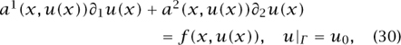
With a little more work one can extend the above discussion to higher-order equations in higher dimensions, and even to systems of equations. Particularly important is the case of a second-order scalar equation in ![]() d,
d,

together with a hypersurface ![]() in
in ![]() d defined by the equation ψ(x) = 0, where ψ is a function with nonvanishing gradient Dψ. Define the unit normal at a point x0 ∈
d defined by the equation ψ(x) = 0, where ψ is a function with nonvanishing gradient Dψ. Define the unit normal at a point x0 ∈ ![]() to be n = Dψ/|Dψ|, or, in component form, ni = ∂iψ/|∂ψ|. As initial conditions for (32) we prescribe the values of u and its normal derivative n[u](x) = n1(x)∂1u(x) + n2(x)∂2u(x) + ··· + nd(x)∂du(x) on
to be n = Dψ/|Dψ|, or, in component form, ni = ∂iψ/|∂ψ|. As initial conditions for (32) we prescribe the values of u and its normal derivative n[u](x) = n1(x)∂1u(x) + n2(x)∂2u(x) + ··· + nd(x)∂du(x) on ![]() :
:
u(x) = u0(x), n[u](x) = u1(x), x ∈ ![]() .
.
It can be shown that ![]() is noncharecteristic (with respect to equation (32)) at a point
is noncharecteristic (with respect to equation (32)) at a point ![]() (that is, we can determine all derivatives of u at
(that is, we can determine all derivatives of u at ![]() in terms of the initial data u0, u1) if and only if
in terms of the initial data u0, u1) if and only if

On the other hand, ![]() is a characteristic hypersurface for (32) if
is a characteristic hypersurface for (32) if

for every x in ![]() .
.
Example. If the coefficients a of (32) satisfy the condition

then clearly, by (34), no surface in ![]() d can be characteristic. This is the case, in particular, for the Laplace equation Δu = f. Consider also the minimal surface equation (7) written in the form
d can be characteristic. This is the case, in particular, for the Laplace equation Δu = f. Consider also the minimal surface equation (7) written in the form
![]()
with h11(∂u) = 1 + (∂2u)2, h22(∂u) = 1 + (∂1u)2, h12(∂u) = h21(∂u) = -∂1u∂2u. It is easy to check that the quadratic form associated with the symmetric matrix hij(∂u) is positive definite for every ∂u. Indeed,
hij(∂u)ξiξj = (1 + |∂u|2)-1/2(|ξ|2 - (1 + |∂u|2)-1(ξ · ∂u)2) > 0.
Thus, even though (36) is not linear, we see that all surfaces in ![]() 2 are noncharacteristic.
2 are noncharacteristic.
Example. Consider the wave equation ![]() u = f in
u = f in ![]() 1+d. All hypersurfaces of the form ψ(t, x) = 0 for which
1+d. All hypersurfaces of the form ψ(t, x) = 0 for which

are characteristic. This is the famous eikonal equation, which plays a fundamental role in the study of wave propagation. Observe that it splits into two Hamilton-Jacobi equations (see (24)):

The bicharacteristic curves of the associated Hamiltonians are called bicharacteristic curves of the wave equation. As particular solutions of (37) we find ψ(t, x) = (t - t0) + |x - x0| and ∂-(t,x) = (t - t0) - |x - x0|, whose level surfaces ∂± = 0 correspond to forward and backward light cones with their vertex at ![]() = (t0, x0). These represent, physically, the union of all light rays emanating from a point source at
= (t0, x0). These represent, physically, the union of all light rays emanating from a point source at ![]() . The light rays are given by the equation (t - t0)ω = (x - x0), for ω ∈
. The light rays are given by the equation (t - t0)ω = (x - x0), for ω ∈ ![]() 3 with |ω| = 1, and are precisely the (t, x) components of the bicharacteristic curves of the Hamilton-Jacobi equations (38). More generally, the characteristics of the linear wave equation
3 with |ω| = 1, and are precisely the (t, x) components of the bicharacteristic curves of the Hamilton-Jacobi equations (38). More generally, the characteristics of the linear wave equation
![]()
with a00 > 0 and aij satisfying (35), are given by the Hamilton-Jacobi equations:
-a00(t, x)(∂tψ)2 + aij(x)∂iψ∂jψ = 0
or, equivalently,

The bicharacteristics of the corresponding Hamiltonian systems are called bicharacteristic curves of (39).
Remark. In the case of the first-order scalar equations (17) we have seen how knowledge of characteristics can be used to find, implicitly, general solutions. We have also seen that singularities propagate only along characteristics. In the case of second-order equations the characteristics are not sufficient to solve the equations, but they continue to provide important information, such as how the singularities propagate. For example, in the case of the wave equation ![]() u = 0 with smooth initial data u0, u1 everywhere except at a point
u = 0 with smooth initial data u0, u1 everywhere except at a point ![]() = (t0, x0), the solution u has singularities present at all points of the light cone -(t - t0)2 + |x - x0|2 = 0 with vertex at
= (t0, x0), the solution u has singularities present at all points of the light cone -(t - t0)2 + |x - x0|2 = 0 with vertex at ![]() . A more refined version of this fact shows that the singularities propagate along bicharacteristics. The general principle here is that singularities propagate along characteristic hypersurfaces of a PDE. Since this is a very important principle, it pays to give it a more precise formulation that extends to general boundary conditions, such as the Dirichlet condition for (1).
. A more refined version of this fact shows that the singularities propagate along bicharacteristics. The general principle here is that singularities propagate along characteristic hypersurfaces of a PDE. Since this is a very important principle, it pays to give it a more precise formulation that extends to general boundary conditions, such as the Dirichlet condition for (1).
Propagation of singularities. If the boundary conditions or the coefficients of a PDE are singular at some point ![]() , and otherwise smooth (or real analytic) everywhere in some small neighborhood V of
, and otherwise smooth (or real analytic) everywhere in some small neighborhood V of ![]() , then a solution of the equation cannot be singular in V except along a characteristic hypersurface passing through
, then a solution of the equation cannot be singular in V except along a characteristic hypersurface passing through ![]() . In particular, if there are no such characteristic hypersurfaces, then any solution of the equation must be smooth (or real analytic) at every point of V other than
. In particular, if there are no such characteristic hypersurfaces, then any solution of the equation must be smooth (or real analytic) at every point of V other than ![]() .
.
Remarks. (i) The heuristic principle mentioned above is invalid, in general, at large scales. Indeed, as we have shown in the case of the Burgers equation, solutions to nonlinear evolution equations can develop new singularities whatever the smoothness of the initial conditions. Global versions of the principle can be formulated for linear equations based on the bicharacteristics of the equation. See (iii) below.
(ii) According to the principle, it follows that any solution of the equation Δu = f, satisfying the boundary condition u|∂D = u0 with a boundary value u0 that merely has to be continuous, is automatically smooth everywhere in the interior of D provided that f itself is smooth there. Moreover, the solution is real analytic if f is real analytic.
(iii) More precise versions of this principle, which plays a fundamental role in the general theory, can be given for linear equations. In the case of the general wave equation (39), for example, one can show that singularities propagate along bicharacteristics. These are the bicharacteristic curves associated with the Hamilton-Jacobi equation (40).
2.4 The Cauchy-Kovalevskaya Theorem
In the case of ODEs we have seen that a noncharacteristic IVP always admits solutions locally (that is, in some time interval about a given point). Is there a higher- dimensional analogue of this fact? The answer is yes, provided that we restrict ourselves to the real-analytic situation, which is covered by an appropriate extension of the Cauchy-Kovalevskaya theorem. More precisely, one can consider general quasilinear equations, or systems, with real-analytic coefficients, real-analytic hypersurfaces ![]() , and appropriate real-analytic initial data on
, and appropriate real-analytic initial data on ![]() .
.
Theorem (Cauchy-Kovalevskaya (CK)). If all the real-analyticity conditions made above are satisfied and if the initial hypersurface ![]() is noncharacteristic at x0,4 then in some neighborhood of x0 there is a unique real-analytic solution u(x) that satisfies the system of equations and the corresponding initial conditions.
is noncharacteristic at x0,4 then in some neighborhood of x0 there is a unique real-analytic solution u(x) that satisfies the system of equations and the corresponding initial conditions.
In the special case of linear equations, an important companion theorem, due to Holmgren, asserts that the analytic solution given by the CK theorem is unique in the class of all smooth solutions and smooth noncharacteristic hypersurfaces ![]() . The CK theorem shows that, given the noncharacteristic condition and the analyticity assumptions, the following straightforward way of finding solutions works: look for a formal expansion of the kind u(x) = ΣαCα(x - x0)α by determining the constants Cα recursively from simple algebraic formulas arising from the equation and initial conditions on
. The CK theorem shows that, given the noncharacteristic condition and the analyticity assumptions, the following straightforward way of finding solutions works: look for a formal expansion of the kind u(x) = ΣαCα(x - x0)α by determining the constants Cα recursively from simple algebraic formulas arising from the equation and initial conditions on ![]() . More precisely, the theorem ensures that the naive expansion obtained in this way converges in a small neighborhood of x0 ∈
. More precisely, the theorem ensures that the naive expansion obtained in this way converges in a small neighborhood of x0 ∈ ![]() .
.
It turns out, however, that the analyticity conditions required by the CK theorem are much too restrictive, and therefore the apparent generality of the result is misleading. A first limitation becomes immediately apparent when we consider the wave equation ![]() u = 0. A fundamental feature of this equation is finite speed of propagation, which means, roughly speaking, that if at some time t a solution u is zero outside some bounded set, then the same must be true at all later times. However, analytic functions cannot have this property unless they are identically zero (see SOME FUNDAMENTAL MATHEMATICAL DEFINITIONS [I.3 §5.6]). Therefore, it is impossible to discuss the wave equation properly within the class of real-analytic solutions. A related problem, first pointed out by HADAMARD [VI.65], concerns the impossibility of solving the Cauchy problem, in many important cases, for arbitrary smooth nonanalytic data. Consider, for example, the Laplace equation Δu = 0 in
u = 0. A fundamental feature of this equation is finite speed of propagation, which means, roughly speaking, that if at some time t a solution u is zero outside some bounded set, then the same must be true at all later times. However, analytic functions cannot have this property unless they are identically zero (see SOME FUNDAMENTAL MATHEMATICAL DEFINITIONS [I.3 §5.6]). Therefore, it is impossible to discuss the wave equation properly within the class of real-analytic solutions. A related problem, first pointed out by HADAMARD [VI.65], concerns the impossibility of solving the Cauchy problem, in many important cases, for arbitrary smooth nonanalytic data. Consider, for example, the Laplace equation Δu = 0 in ![]() d. As we have established above, any hypersurface
d. As we have established above, any hypersurface ![]() is noncharacteristic, yet the Cauchy problem u|
is noncharacteristic, yet the Cauchy problem u|![]() = u0, n[u]|
= u0, n[u]|![]() = u1, for arbitrary smooth initial conditions u0, u1, may admit no local solutions in a neighborhood of any point of
= u1, for arbitrary smooth initial conditions u0, u1, may admit no local solutions in a neighborhood of any point of ![]() . Indeed, take
. Indeed, take ![]() to be the hyperplane x1 = 0 and assume that the Cauchy problem can be solved for given nonanalytic smooth data in a domain that includes a closed ball B centered at the origin. The corresponding solution can also be interpreted as the solution to the Dirichlet problem in B, with the values of u prescribed on the boundary ∂B. But this, according to our heuristic principle (which can easily be made rigorous in this case), must be real analytic everywhere in the interior of B, contradicting our assumptions about the initial data.
to be the hyperplane x1 = 0 and assume that the Cauchy problem can be solved for given nonanalytic smooth data in a domain that includes a closed ball B centered at the origin. The corresponding solution can also be interpreted as the solution to the Dirichlet problem in B, with the values of u prescribed on the boundary ∂B. But this, according to our heuristic principle (which can easily be made rigorous in this case), must be real analytic everywhere in the interior of B, contradicting our assumptions about the initial data.
On the other hand, the Cauchy problem for the wave equation ![]() u = 0 in
u = 0 in ![]() d+1 has a unique solution for any smooth initial data u0, u1 that is prescribed on a spacelike hypersurface. This means a hypersurface ψ(t, x) = 0 such that at every point
d+1 has a unique solution for any smooth initial data u0, u1 that is prescribed on a spacelike hypersurface. This means a hypersurface ψ(t, x) = 0 such that at every point ![]() = (t0, x0) that belongs to it the normal vector at
= (t0, x0) that belongs to it the normal vector at ![]() lies inside the light cone (either in the future direction or in the past direction). To say this analytically,
lies inside the light cone (either in the future direction or in the past direction). To say this analytically,

This condition is clearly satisfied by a hyperplane of the form t = t0, but any other hypersurface close to this is also spacelike. By contrast, the IVP is ill-posed for a timelike hypersurface, i.e., a hypersurface for which

That is, we cannot, for general non-real-analytic initial conditions, find a solution of the IVP. An example of a timelike hypersurface is given by the hyperplane x1 = 0. Let us explain the term “ill-posed” more precisely.
Definition. A given problem for a PDE is said to be well-posed if both existence and uniqueness of solutions can be established for arbitrary data that belongs to a specified large space of functions, which includes the class of smooth functions.5 Moreover, the solutions must depend continuously on the data. A problem that is not well-posed is called ill-posed.
The continuous dependence on the data is very important. Indeed, the IVP would be of little use if very small changes in the initial conditions resulted in very large changes in the corresponding solutions.
2.5 Standard Classification
The different behavior of the Laplace and wave equations mentioned above illustrates the fundamental difference between ODEs and PDEs and the illusory generality of the CK theorem. Given that these two equations are so important in geometric and physical applications, it is of great interest to find the broadest classes of equations with which they share their main properties. The equations modeled by the Laplace equation are called elliptic, while those modeled by the wave equation are called hyperbolic. The other two important models are the heat equation (see (2)) and the Schrödinger equation (see (4)). The general classes of equations that they resemble are called parabolic and dispersive, respectively.
Elliptic equations are the most robust and the easiest to characterize: they are the ones that admit no characteristic hypersurfaces.
Definition. A linear, or quasilinear, N × N system with no characteristic hypersurfaces is called elliptic.
Equations of type (32) whose coefficients aij satisfy condition (35) are clearly elliptic. The minimal surface equation (7) is also elliptic. It is also easy to verify that the Cauchy-Riemann system (12) is elliptic. As was pointed out by Hadamard, the IVP is not well-posed for elliptic equations. The natural way of parametrizing the set of solutions to an elliptic PDE is to prescribe conditions for u, and some of its derivatives (the number of derivatives will be roughly half the order of the equation) at the boundary of a domain D ⊂ ![]() n. These are called boundary-value problems (BVPs). A typical example is the Dirichlet boundary condition u|∂D = u0 for the Laplace equation Δu = 0 in a domain D ⊂
n. These are called boundary-value problems (BVPs). A typical example is the Dirichlet boundary condition u|∂D = u0 for the Laplace equation Δu = 0 in a domain D ⊂ ![]() n. One can show that, if the domain D satisfies certain mild regularity assumptions and the boundary value u0 is continuous, then this problem admits a unique solution that depends continuously on u0. We say that the Dirichlet problem for the Laplace equation is well-posed. Another well-posed problem for the Laplace equation is given by the Neumann boundary condition n[u]|∂D = f, where n is the exterior unit normal to the boundary. This problem is well-posed for all continuous functions f defined on ∂D with zero mean average. A typical problem of general theory is to classify all well-posed BVPs for a given elliptic system.
n. One can show that, if the domain D satisfies certain mild regularity assumptions and the boundary value u0 is continuous, then this problem admits a unique solution that depends continuously on u0. We say that the Dirichlet problem for the Laplace equation is well-posed. Another well-posed problem for the Laplace equation is given by the Neumann boundary condition n[u]|∂D = f, where n is the exterior unit normal to the boundary. This problem is well-posed for all continuous functions f defined on ∂D with zero mean average. A typical problem of general theory is to classify all well-posed BVPs for a given elliptic system.
As a consequence of our propagation-of-singularities principle, we deduce, heuristically at least, the following general fact:
Classical solutions of elliptic equations with smooth (or real-analytic) coefficients in a regular domain D are smooth (or real analytic) in the interior of D, whatever the degree of smoothness of the boundary conditions.6
Hyperbolic equations are, essentially, those for which the IVP is well-posed. In that sense, they provide the natural class of equations for which one can prove a result similar to the local existence theorem for ODEs. More precisely, for each sufficiently regular set of initial conditions there is a unique solution. We can thus think of the Cauchy problem as a natural way of parametrizing the set of all solutions to the equations.
The definition of hyperbolicity depends, however, on the particular hypersurface we are considering as the initial hypersurface. Thus, in the case of the wave equation ![]() u = 0, the standard IVP
u = 0, the standard IVP
u(0, x) = u0(x), ∂tu(0, x) = u1
is well-posed. This means that for any smooth initial data u0, u1 we can find a unique solution of the equation, which depends continuously on u0, u1. As we have already mentioned, the IVP for ![]() u = 0 remains well-posed if we replace the initial hypersurface t = 0 by any spacelike hypersurface ψ(t, x) = 0 (see (41)). However, it fails to be well-posed for timelike hypersurfaces, for which there may be no solution with prescribed, nonanalytic, Cauchy data.
u = 0 remains well-posed if we replace the initial hypersurface t = 0 by any spacelike hypersurface ψ(t, x) = 0 (see (41)). However, it fails to be well-posed for timelike hypersurfaces, for which there may be no solution with prescribed, nonanalytic, Cauchy data.
It is more difficult to give algebraic conditions for hyperbolicity. Roughly speaking, hyperbolic equations are at the opposite end of the spectrum from elliptic equations: whereas elliptic equations have no characteristic hypersurfaces, hyperbolic equations have as many as possible passing through any given point. One of the most useful classes of hyperbolic equations, which includes most of the important known examples, consists of equations of the form

where all the coefficients A0, A1, . . . , Ad are symmetric N × N matrices and ![]() is given by ψ(t, x) = 0. Such a system is well-posed provided that the matrix
is given by ψ(t, x) = 0. Such a system is well-posed provided that the matrix

is positive definite. A system (42) that satisfies these conditions is called symmetric hyperbolic. In the particular case when ψ(t, x) = t, the condition (43) becomes
(A0ξ,ξ) ≥ c|ξ|2 ∀ξ ∈ ![]() N.
N.
The following is a fundamental result in the theory of general hyperbolic equations. It is called the local existence and uniqueness of solutions for symmetric hyperbolic systems.
Theorem (fundamental theorem for hyperbolic equations). The IVP (42) is locally well posed for symmetric hyperbolic systems with sufficiently smooth A, F, and ![]() and sufficiently smooth initial conditions u0. In other words, if the appropriate smoothness conditions are satisfied, then for any point
and sufficiently smooth initial conditions u0. In other words, if the appropriate smoothness conditions are satisfied, then for any point ![]() ∈
∈ ![]() there is a small neighborhood D of
there is a small neighborhood D of ![]() 7 inside which there is a unique, continuously differentiable solution u.
7 inside which there is a unique, continuously differentiable solution u.
Remarks. (I) The local character of the theorem is essential, just as it was for the general propagation-of-singularities principle discussed earlier, since the result cannot be globalized in the particular case of the Burgers equation (21), which fits trivially into the framework of general nonlinear symmetric hyperbolic systems. A precise version of the theorem above gives a lower bound on how large ![]() can be.
can be.
(ii) The proof of the theorem is based on a variation of the Picard iteration method that we encountered earlier for ODEs. One starts by taking u(0) = u0 in a neighborhood of ![]() . Then one defines functions u(n) recursively as follows:
. Then one defines functions u(n) recursively as follows:

Notice that at each stage of the iteration we have to solve a linear equation. Linearization is an extremely important tool in studying nonlinear PDEs. We can almost never understand their behavior without linearizing them around important special solutions. Thus, almost invariably, hard problems in nonlinear PDEs reduce to understanding specific problems in linear PDEs.
(ill) To implement the Picard iteration method we need to get precise estimates concerning u(n) in terms of u(n-1). This step requires energy type a priori estimates, which we will discuss in section 3.3.
Another important property of hyperbolic equations (which is not shared by elliptic, parabolic, or dispersive equations) is finite speed of propagation, which was mentioned earlier in the case of the wave equation (3). Consider this simple case again. The IVP can be solved explicitly by the so-called Kirchhoff formula. The formula allows us to conclude that if the initial data at t = 0 is zero outside a ball Ba(x0) of radius a > 0 centered at x0 ∈ ![]() 3, then at time t > 0 the solution u is zero outside the ball Ba+ct(x0). In general, finite speed of propagation can best be formulated in terms of domains of dependence and influence of hyperbolic equations (see the online version for general definitions).
3, then at time t > 0 the solution u is zero outside the ball Ba+ct(x0). In general, finite speed of propagation can best be formulated in terms of domains of dependence and influence of hyperbolic equations (see the online version for general definitions).
Hyperbolic PDEs play a fundamental role in physics, as they are intimately tied to the relativistic nature of the modern theory of fields. Equations (3), (5), (13) are the simplest examples of linear field theories, and they are manifestly hyperbolic. Other basic examples appear in gauge field theories such as MAXWELL’S EQUATIONS [IV.13 §1.1] ∂αFαβ = 0 or the Yang-Mills equations DαFαβ = 0. Finally, the Einstein equations (14) are also hyperbolic.8 Other important examples of hyperbolic equations arise in the physics of elasticity and inviscid fluids. As examples of the latter, the Burgers equation (21) and the compressible Euler equation are hyperbolic.
Elliptic equations, on the other hand, appear naturally in describing time-independent, or more generally steady-state, solutions of hyperbolic equations Elliptic equations can also be derived, directly, by well-defined VARIATIONAL PRINCIPLES [III.94].
Finally, a few words about parabolic equations and Schrödinger-type equations, which are intermediate between the elliptic and hyperbolic ones. Large classes of useful equations of these types are given by
![]()
and
![]()
respectively, where L is an elliptic second-order operator. One looks for solutions u = u(t, x), defined for t ≥ t0, with the prescribed initial condition
![]()
on the hypersurface t = t0. Strictly speaking, this hypersurface is characteristic, since the order of the equation is 2 and we cannot determine ![]() at t = t0 directly from the equation. Yet this is not a serious problem; we can still determine
at t = t0 directly from the equation. Yet this is not a serious problem; we can still determine ![]() formally by differentiating the equation with respect to ∂t. Thus, the IVP (44) (or (45)) with initial condition (46) is well-posed, but not quite in the same sense as for hyperbolic equations. For example, the heat equation -∂tu + Δu is well-posed for positive t but ill-posed for negative t. The heat equation may also not have unique solutions for the IVP unless we make assumptions about how fast the initial data is allowed to grow at infinity. One can also show that the characteristic hypersurfaces of the equation (44) are all of the form, and therefore parabolic equations are quite similar to elliptic equations. For example, one can show that if the coefficients aij and f are smooth (or real analytic), then the solution u must be smooth (or real analytic in x) for t > t0 even if the initial data u0 is not smooth, which is consistent with our propagation-of-singularities principle. The heat equation smooths out initial conditions. It is for this reason that the heat equation is useful in many applications. In physics, parabolic PDEs arise whenever diffusion or dissipation phenomena are important, while in geometry and calculus of variations, parabolic PDEs often arise as gradient flows of positive-definite functionals. Ricci flow (16) can also be viewed as a parabolic PDE, after a suitable change of coordinates.
formally by differentiating the equation with respect to ∂t. Thus, the IVP (44) (or (45)) with initial condition (46) is well-posed, but not quite in the same sense as for hyperbolic equations. For example, the heat equation -∂tu + Δu is well-posed for positive t but ill-posed for negative t. The heat equation may also not have unique solutions for the IVP unless we make assumptions about how fast the initial data is allowed to grow at infinity. One can also show that the characteristic hypersurfaces of the equation (44) are all of the form, and therefore parabolic equations are quite similar to elliptic equations. For example, one can show that if the coefficients aij and f are smooth (or real analytic), then the solution u must be smooth (or real analytic in x) for t > t0 even if the initial data u0 is not smooth, which is consistent with our propagation-of-singularities principle. The heat equation smooths out initial conditions. It is for this reason that the heat equation is useful in many applications. In physics, parabolic PDEs arise whenever diffusion or dissipation phenomena are important, while in geometry and calculus of variations, parabolic PDEs often arise as gradient flows of positive-definite functionals. Ricci flow (16) can also be viewed as a parabolic PDE, after a suitable change of coordinates.
Dispersive PDEs, of which the Schrödinger equation (4) is a fundamental example, are evolution equations that behave analogously to hyperbolic PDEs in many respects. For instance, the IVP tends to be locally well-posed both forward and backward in time. However, solutions to dispersive PDEs do not propagate along characteristic surfaces. Instead, they move at speeds that are determined by their spatial frequency; in general, high-frequency waves tend to propagate at much greater speeds than low-frequency waves, which eventually leads to a dispersion of the solution into increasingly large areas of space. In fact, the speed of propagation of solutions is typically infinite This behavior also differs from that of parabolic equations, which tend to dissipate the high-frequency components of a solution (sending them to zero) rather than dispersing them. In physics, dispersive equations arise in quantum mechanics: they are the nonrelativistic limit c → ∞ of relativistic equations and they are also approximations to model certain types of fluid behavior. For instance, the KORTEWEG-DE VRIES EQUATION [III.49],
![]()
is a dispersive PDE that models the behavior of small-amplitude waves in a shallow canal.
2.6 Special Topics for Linear Equations
The greatest successes of the general theory have been in connection with linear equations, especially those with constant coefficients, for which Fourier analysis provides an extremely powerful tool. While the related issues of classification, well-posedness, and propagation of singularities have dominated the study of linear equations, there are other issues of interest as well, including the following.
2.6.1 Local Solvability
This is the problem of determining the conditions on a linear operator ![]() and given data f under which the equation (9) is locally solvable. The Cauchy-Kovalevskaya theorem gives a criterion for local solvability when f and the coefficients of
and given data f under which the equation (9) is locally solvable. The Cauchy-Kovalevskaya theorem gives a criterion for local solvability when f and the coefficients of ![]() are real analytic, but it is a remarkable phenomenon that when one relaxes this assumption slightly, asking for f to be smooth rather than real analytic, serious obstructions to local solvability appear. For instance, the Lewy operator
are real analytic, but it is a remarkable phenomenon that when one relaxes this assumption slightly, asking for f to be smooth rather than real analytic, serious obstructions to local solvability appear. For instance, the Lewy operator
![]()
defined on complex-valued functions u : ![]() ×
× ![]() →
→ ![]() , has the property that equation (9) is locally solvable for real-analytic f but not for most smooth f. The Lewy operator is intimately connected to the tangential Cauchy-Riemann equations on the Heisenberg group in
, has the property that equation (9) is locally solvable for real-analytic f but not for most smooth f. The Lewy operator is intimately connected to the tangential Cauchy-Riemann equations on the Heisenberg group in ![]() 2. It was discovered in the study of the restriction of the two-dimensional analogue of the Cauchy-Riemann operator
2. It was discovered in the study of the restriction of the two-dimensional analogue of the Cauchy-Riemann operator ![]() to a quadric in
to a quadric in ![]() 2. This example was the starting point for the theory of local solvability, whose goal is to characterize linear equations that are locally solvable. The theory of Cauchy-Riemann manifolds—which has its origin in the study of restrictions of the Cauchy-Riemann equations (in higher dimensions) to real hypersurfaces, each of which comes with an associated “tangential Cauchy-Riemann complex”—is another extremely rich source of examples of interesting linear PDEs, which do not fit into the standard classification.
2. This example was the starting point for the theory of local solvability, whose goal is to characterize linear equations that are locally solvable. The theory of Cauchy-Riemann manifolds—which has its origin in the study of restrictions of the Cauchy-Riemann equations (in higher dimensions) to real hypersurfaces, each of which comes with an associated “tangential Cauchy-Riemann complex”—is another extremely rich source of examples of interesting linear PDEs, which do not fit into the standard classification.
2.6.2 Unique Continuation
This concerns various ill-posed problems where solutions may not always exist, but one still has uniqueness. A fundamental example is that of analytic continuation: two holomorphic functions on a connected domain D that agree on a nondiscrete set (such as a disk or an interval) must necessarily agree everywhere on D. This fact can be viewed as a unique continuation result for the Cauchy-Riemann equations (12). Another example in a similar spirit is Holmgren’s theorem, which asserts that solutions to a linear PDE (9) that has real- analytic coefficients and data are unique, even in the class of smooth functions. More generally, the study of ill-posed problems (such as the wave equation with prescribed data on a timelike surface rather than a space-like one) arises naturally in connection with control theory.
2.6.3 Spectral Theory
There is no way I can even begin to give an account of this theory, which is of fundamental importance not only to quantum mechanics and other physical theories, but also to geometry and ANALYTIC NUMBER THEORY [IV.2]. Just as a matrix A can often be analyzed through its EIGENVALUES AND EIGENVECTORS [I.3 §4.3] by the tools of linear algebra, one can learn much about a linear differential operator ![]() and its associated PDE by understanding that operator’s SPECTRUM [III.86] and eigenfunctions with the help of tools from FUNCTIONAL ANALYSIS [IV.15]. A typical problem in spectral theory is the eigenvalue problem in
and its associated PDE by understanding that operator’s SPECTRUM [III.86] and eigenfunctions with the help of tools from FUNCTIONAL ANALYSIS [IV.15]. A typical problem in spectral theory is the eigenvalue problem in ![]() d:
d:
-Δu(x) + V(x)u(x) = λu(x).
A function u that is localized in space (for example, by being bounded in the L2(![]() d)-norm) and that satisfies this equation is mapped by the linear operator -Δ + V to the function λu: we say that u is an eigenfunction with eigenvalue λ.
d)-norm) and that satisfies this equation is mapped by the linear operator -Δ + V to the function λu: we say that u is an eigenfunction with eigenvalue λ.
Suppose that we have an eigenfunction u and let ϕ(t, x) = e-iλtu(x). It is easy to check that ϕ is a solution of the Schrödinger equation
![]()
Moreover, it has a very special form. Such solutions are called bound states of the physical system described by (47). The eigenvalues λ, which form a discrete set, correspond to the quantum energy levels of the system. They are very sensitive to the choice of potential V. The inverse spectral problem is also important: can one determine the potential V from knowledge of the corresponding eigenvalues? The eigenvalue problem can be studied in considerable generality by replacing the operator -Δ + V with other elliptic operators. For instance, in geometry it is important to study the eigenvalue problem for the Laplace-Beltrami operator, which is the natural generalization of the Laplace operator from ![]() n to general RIEMANNIAN MANIFOLDS [I.3 §6.10]. When the manifold has some arithmetic structure (for instance, if it is the quotient of the upper half-plane by a discrete arithmetic group), this problem is of major importance in number theory, leading, for instance, to the theory of Hecke-Maas forms. A famous problem in differential geometry (“can you hear the shape of a drum?”) is to characterize the metric on a compact surface from the spectral properties of the associated Laplace-Beltrami operator.
n to general RIEMANNIAN MANIFOLDS [I.3 §6.10]. When the manifold has some arithmetic structure (for instance, if it is the quotient of the upper half-plane by a discrete arithmetic group), this problem is of major importance in number theory, leading, for instance, to the theory of Hecke-Maas forms. A famous problem in differential geometry (“can you hear the shape of a drum?”) is to characterize the metric on a compact surface from the spectral properties of the associated Laplace-Beltrami operator.
2.6.4 Scattering Theory
This theory formalizes the intuition from quantum mechanics that a potential which is small or localized is largely unable to “trap” a quantum particle, which is therefore likely to escape to infinity in a manner resembling that of a free particle. In the case of equation (47), solutions that scatter are those that behave freely as t → ∞. That is, they behave like solutions to the free Schrödinger equation i∂tψ + Δψ = 0. A typical problem in scattering theory is to show that, if V(x) tends to zero sufficiently fast as |x| → ∞, all solutions, except the bound states, scatter as t → ∞.
2.7 Conclusions
In the analytic case, the CK theorem allows us to solve the IVP locally for very general classes of PDEs. We have a general theory of characteristic hypersurfaces of PDEs and a good general understanding of how they relate to propagation of singularities. We can also distinguish in considerable generality the fundamental classes of elliptic and hyperbolic equations and can define general parabolic and dispersive equations. The IVP for a large class of nonlinear hyperbolic systems can be solved locally in time, for sufficiently smooth initial conditions. Similar local-in-time results hold for general classes of nonlinear parabolic and dispersive equations. For linear equations a lot more can be done. We have satisfactory results concerning the regularity of solutions for elliptic and parabolic equations and a good understanding of the propagation of singularities for a large class of hyperbolic equations. Some aspects of spectral theory and scattering theory and problems of unique continuation can also be studied in considerable generality.
The main defect of the general theory concerns the passage from local to global. Important global features of special equations are too subtle to fit into a general scheme. Rather, each important PDE requires special treatment. This is particularly true for nonlinear equations: the long-term behavior of solutions is very sensitive to the special features of the equation at hand. Moreover, general points of view may obscure, through unnecessary technical complications, the main properties of the important special cases. A useful general framework is one that provides a simple and elegant treatment of a particular phenomenon, as is the case for symmetric hyperbolic systems and the phenomenon of local well-posedness and finite speed of propagation. However, it turns out that symmetric hyperbolic systems are simply too general for the study of more refined questions about the important examples of hyperbolic equations.
3 General Ideas
As one turns away from the general theory, one may be inclined to accept the pragmatic point of view described earlier, according to which PDEs is not a real subject but is rather a collection of subjects such as hydrodynamics, general relativity, several complex variables, elasticity, etc., each organized around a special equation. However, this rather widespread viewpoint has its own serious drawbacks. Even though specific equations have specific properties, the tools that are used to derive them are intimately related. In fact, there is an impressive body of knowledge relevant to all important equations, or at least large classes of them. Lack of space does not allow me to do anything more than enumerate them below.9
3.1 Well-Posedness
As is clear from the previous section, well-posed problems are at the heart of the modern theory of PDEs. Recall that these are problems that admit unique solutions for given smooth initial or boundary conditions, and that the corresponding solutions have to depend continuously on the data. It is this condition that leads to the classification of PDEs into elliptic, hyperbolic, parabolic, and dispersive equations. The first step in the study of a nonlinear evolution equation is a proof of a local-in-time existence and uniqueness theorem, similar to the one for ODEs. Ill-posedness, the counterpart of well-posedness, is also important in many applications. The Cauchy problem for the wave equation (3), with data on the timelike hypersurface z = 0, is a typical example. Ill-posed problems appear naturally in control theory, as we have mentioned, and also in inverse scattering.
3.2 Explicit Representations and Fundamental Solutions
Our basic equations (2)-(5) can be solved explicitly. For example, the solution to the IVP for the heat equation in ![]() , that is, the problem of finding a function u that satisfies
, that is, the problem of finding a function u that satisfies
-∂tu + Δu = 0, u(0, x) = u0(x),
for t ≥ 0, is given by
![]()
for a certain function Ed, which is called the fundamental solution of the heat operator -∂t + Δ. This function can be defined explicitly: when t ≤ 0 it is 0, and when t > 0 it is given by the formula Ed(t, x) = (4πt)-d/2e-|X|2/4t. Observe that Ed satisfies the equation (-∂t + Δ)E = 0 in both regions t < 0 and t > 0, but it has a singularity at t = 0, which prevents it from satisfying the equation in the whole of ![]() 1+d. In fact, we can check that for any function10
1+d. In fact, we can check that for any function10 ![]() we have
we have

In the language of DISTRIBUTION THEORY [III.18], formula (48) means that Ed, as a distribution, satisfies the equation (-∂t + Δ)Ed = δ0, where δ0 is the Dirac distribution in ![]() 1+d supported at the origin. That is,
1+d supported at the origin. That is, ![]() . A similar notion of fundamental solution can be defined for the Poisson, wave, Klein-Gordon, and Schrödinger equations.
. A similar notion of fundamental solution can be defined for the Poisson, wave, Klein-Gordon, and Schrödinger equations.
A powerful method of solving linear PDEs with constant coefficients is based on THE FOURIER TRANSFORM [III.27]. For example, consider the heat equation ∂t - Δu = 0 in one space dimension, with initial condition u(0, x) = u0. Define û(t, ξ) to be the Fourier transform of u relative to the space variable:
![]()
It is easy to see that û(t, ξ) satisfies the differential equation
∂tû(t, ξ) = -ξ2û(t, ξ), û(0, ξ) = û0(ξ).
This can be solved by a simple integration, which results in the formula û(t, ξ) = û0(ξ)e-t|ξ|2. Thus, with the help of the inverse Fourier transform, we derive a formula for u(t, x):
![]()
Similar formulas can be derived for our other basic evolution equations. For example, in the case of the wave equation ![]() in three dimensions, subject to the initial data u(0, x) = u0, ∂tu(0, x) = 0, we find that
in three dimensions, subject to the initial data u(0, x) = u0, ∂tu(0, x) = 0, we find that
![]()
After some work, one can reexpress formula (49) in the form
![]()
where da is the area element of the sphere |x - y| = t of radius t centered at x. This is the well-known Kirchhoff formula. By contrast with (49), the integration here is with respect to the physical variables t and x only. It is instructive to compare these two formulas. Using the Plancherel identity it is very easy to deduce from (49) the L2 bound
![]()
while the possibility of obtaining such a bound from (50) seems unlikely since the formula involves a derivative. On the other hand, (50) is perfect for giving us information about the domain of influence. Indeed, we can see immediately from the formula that if u0 is zero outside the ball Ba = {|x - x0| ≤ a}, then u(t,x) is zero outside the ball Ba+|t| for any time t. This fact does not seem at all transparent in the Fourier-based formula (49). The fact that different representations of solutions have different, even opposite, strengths and weaknesses has important consequences for constructing approximate solutions, or parametrices, for more complicated equations, such as linear equations with variable coefficients or nonlinear wave equations. There are two possible types of constructions: those in physical space, which mimic the physical-space formula (50), and those in Fourier space, which mimic the formula (49).
3.3 A Priori Estimates
Most equations cannot be solved explicitly. However, if we are interested in qualitative information about a solution, then it is not necessary to derive it from an exact formula. But how else, one might wonder, can we extract such information? A priori estimates are a very important technique for doing this.
The best-known examples are energy estimates, the maximum principle, and monotonicity arguments. The simplest example of the first type is the following identity (which is a very simple example of a so-called Bochner-type identity):
![]()
The left-hand side is shorthand for
![]()
and the identity holds for all functions u that are twice continuously differentiable and tend to zero as |x| → ∞. This formula can be justified fairly simply by integrating by parts. As a consequence of the Bochner identity, we obtain the a priori estimate that if u is a smooth solution to the Poisson equation (6) with square-integrable data f, and if it tends to zero at infinity, then the square integral of its second derivatives is bounded:
![]()
Thus we obtain the qualitative fact that, on average (in a mean-square sense), u has “two more degrees of regularity” than f.11 This is called an energy-type estimate because, in physical situations, the square of the L2-norm can often be interpreted as some type of kinetic energy.
The Bochner identity can be extended to more general Riemannian manifolds than ![]() d, although one then picks up some additional lower-order terms involving the curvature of those manifolds. Such identities play a major role in the theory of geometric PDEs on these manifolds.
d, although one then picks up some additional lower-order terms involving the curvature of those manifolds. Such identities play a major role in the theory of geometric PDEs on these manifolds.
Energy-type identities and estimates also exist for parabolic, dispersive, and hyperbolic PDEs. For instance, they play a fundamental role in demonstrating the local existence, uniqueness, and finite speed of propagation for hyperbolic PDEs with smooth initial data. Energy estimates become particularly powerful when combined with inequalities such as the Sobolev embedding inequality, which allows one to convert the “L2” information provided by these estimates into pointwise (or “L∞”) type information (see FUNCTION SPACES [III.29 §§2.4, 3]).
While energy identities and L2 estimates (which, as in the above example, come from integration by parts) apply to all, or at least major classes of, PDEs, the maximum principle can be applied only to elliptic and parabolic PDEs. The following theorem is the simplest manifestation of it. Note that the theorem provides us with important quantitative information about solutions to the Laplace equation even in the absence of any explicit representation for them.
Theorem (maximum principle). Assume that u is a solution to the Laplace equation (1) on a bounded connected domain D ∈ ![]() d with a smooth boundary ∂D. Assume also that u is continuous on the closure of D and has continuous first and second partial derivatives in the interior of D. Then u must achieve its maximum and minimum values on the boundary. Moreover, if the maximum or minimum is also achieved at an interior point of D, then u must be constant in D.
d with a smooth boundary ∂D. Assume also that u is continuous on the closure of D and has continuous first and second partial derivatives in the interior of D. Then u must achieve its maximum and minimum values on the boundary. Moreover, if the maximum or minimum is also achieved at an interior point of D, then u must be constant in D.
The method is very robust and can easily be extended to a large class of second-order elliptic equations. It can also be extended to parabolic equations and systems, and plays a crucial role in, for example, the study of Ricci flow.
Let us briefly mention some other important classes of a priori estimates. The Sobolev inequalities, which are of prime importance in elliptic equations, have several counterparts in linear and nonlinear hyperbolic and dispersive equations, including the Strichartz estimates and bilinear estimates. In connection with ill-posed problems and unique continuation, Carle- man estimates play a fundamental role. Finally, several a priori estimates arising from monotonicity formulas12—such as virial identities, Pohozaev identities, or Morawetz inequalities—can be used to establish the breakdown of regularity or the blow-up of solutions to some nonlinear equations, and to guarantee global existence and decay of solutions to others.
To summarize, it is not much of an exaggeration to say that a priori estimates play a fundamental role in more or less every aspect of the modern theory of PDEs.
3.4 Bootstrap and Continuity Arguments
The bootstrap argument is a method, or rather a powerful general philosophy, to derive a priori estimates for nonlinear equations. According to this philosophy we start by making educated assumptions about the solutions we are trying to describe. These assumptions allow us to think of the original nonlinear problem as a linear one whose coefficients satisfy properties consistent with the assumptions. We may then use linear methods, based on other a priori estimates that we already know, to try to show that the solutions to this linear problem behave as well as we have postulated—in fact, even better. One can characterize this powerful method, which allows us to use linear theory without actually having to linearize the equation, as a conceptual linearization. It can also be regarded as a continuity argument relative to some parameter, which might be the natural time parameter of an evolution problem, but it could also be an artificial parameter which we have the freedom to introduce ourselves. This latter situation is typical of applications to nonlinear elliptic equations. In the online version of this article we provide a few examples to illustrate the method in both cases.
3.5 The Method of Generalized Solutions
Since a PDE involves differentiation, it might seem obvious that in any discussion of PDEs we should restrict our attention to differentiable functions. However, it is possible to generalize the notion of differentiation so that it makes sense for a wider class of functions, and even for function-like objects, such as distributions, that are not functions at all. This allows us to make sense of a PDE in a broader context, and admits the possibility of generalized solutions.
The best way to introduce generalized solutions in PDEs and explain why they are important is through the Dirichlet principle. This originates in the observation that, out of all functions that are defined on a bounded domain D ⊂ ![]() d, that satisfy prescribed Dirichlet boundary condition u|∂D = f, and that live in an appropriate functional space X, the functions u that minimize the Dirichlet integral (or Dirichlet functional)
d, that satisfy prescribed Dirichlet boundary condition u|∂D = f, and that live in an appropriate functional space X, the functions u that minimize the Dirichlet integral (or Dirichlet functional)

are the harmonic functions (that is, solutions of the equation Δu = 0). It was RIEMANN [VI.49] who first had the idea of trying to use this fact to solve the Dirichlet problem: in order to find a solution u to the problem
![]()
one should find (by some means other than solving the Dirichlet problem) a function u that minimizes the Dirichlet integral while equaling u0 on ∂D. To do this, one must specify the set by functions, or rather the function space, over which the minimization is taking place. The history of how this choice was made is a fascinating one. A natural choice is X = C1(![]() ), the space of continuously differentiable functions on
), the space of continuously differentiable functions on ![]() , where the norm of a function υ is
, where the norm of a function υ is
![]()
In particular, the Dirichlet norm ||υ||Dr is finite when υ belongs to this space. In fact, Riemann chose X = C2(![]() ) (a similar space but designed for twice continuously differentiable functions). This bold but flawed attempt was followed by a penetrating criticism by WEIERSTRASS [VI.44], who showed that the functional does not have to achieve its minimum in either C2(
) (a similar space but designed for twice continuously differentiable functions). This bold but flawed attempt was followed by a penetrating criticism by WEIERSTRASS [VI.44], who showed that the functional does not have to achieve its minimum in either C2(![]() ) or C1(
) or C1(![]() ). However, Riemann’s basic idea was revived, and it eventually triumphed after a long and inspiring process that involved defining appropriate function spaces, introducing the notion of generalized solutions, and developing a regularity theory for them. (The precise formulation of the Dirichlet principle also requires the definition of SOBOLEV SPACES [III.29 §2.4].)
). However, Riemann’s basic idea was revived, and it eventually triumphed after a long and inspiring process that involved defining appropriate function spaces, introducing the notion of generalized solutions, and developing a regularity theory for them. (The precise formulation of the Dirichlet principle also requires the definition of SOBOLEV SPACES [III.29 §2.4].)
Let us briefly summarize the method, which has since been vastly extended so that it can be applied to a large class of linear13 and nonlinear elliptic and parabolic equations. It is based on two steps. In the first step one applies a minimization procedure. Although, as Weierstrass discovered, the natural function spaces may not contain functions that achieve the minimum, one can use such a procedure to find a generalized solution instead. This may not seem very interesting, since we were looking for a function that solves the Dirichlet problem (or one of the other problems to which the method can be applied). But this is where the second step comes in: it is sometimes possible to show that the generalized solution must in fact be a classical solution (that is, an appropriately smooth function) after all. This is the “regularity theory” mentioned earlier. In some situations, however, the generalized solution may turn out to have singularities and therefore not be regular. Then the challenge is to understand the nature of these singularities and to prove realistic partial regularity results. For instance, it is sometimes possible to prove that the generalized solution is smooth everywhere apart from in a small “exceptional set.”
Though generalized solutions are at their most effective for elliptic problems, their range of applicability encompasses all PDEs. For example, we have already seen that the fundamental solutions to the basic linear equations have to be interpreted as distributions, which are examples of generalized solutions.
The notion of generalized solutions has also proved successful for nonlinear evolution problems, such as systems of conservation laws in one space dimension. An excellent example is provided by the Burgers equation (21). As we have seen, solutions to ∂tu + u∂xu = 0 develop singularities in finite time no matter how smooth the initial conditions are. It is natural to ask whether solutions continue to make sense, as generalized solutions, even beyond the time when these singularities form. A natural notion of generalized solution is a function u such that
![]()
for every smooth function ϕ that is zero outside a bounded set, since one can make sense of the integral even when u is not a differentiable function. Integrating this by parts (the first term with respect to t and the second with respect to x) one obtains the following formulation:
![]()
It can be shown that, under additional conditions called entropy conditions, the IVP for the Burgers equation admits a unique generalized solution that is global: that is, valid for every t ∈ ![]() . Today we have a satisfactory theory of global solutions to a large class of hyperbolic systems of one-dimensional “conservation laws.” These systems, for which the above-mentioned theory applies, are called strictly hyperbolic.
. Today we have a satisfactory theory of global solutions to a large class of hyperbolic systems of one-dimensional “conservation laws.” These systems, for which the above-mentioned theory applies, are called strictly hyperbolic.
For more complicated nonlinear evolution equations, the question of what constitutes a good concept of a generalized solution, though fundamental, is far murkier. For higher-dimensional evolution equations the first concept of a weak solution was introduced by Leray. Let us call a generalized solution weak if one cannot prove any type of uniqueness for it. This unsatisfactory situation may be temporary, i.e., the result of our technical inabilities, or unavoidable, in the sense that the concept itself is flawed. Leray was able to produce, by a compactness method, a weak solution of the IVP for the NAVIER-STOKES EQUATIONS [III.23]. The great advantage of the compactness method (and its modern extensions, which can, in some cases, cleverly circumvent lack of compactness) is that it produces global solutions for all data. This is particularly important for supercritical or critical nonlinear evolution equations, which we will discuss later. For these we expect classical solutions to develop singularities in a finite time. The problem, however, is that one has very little control over such solutions. In particular, we do not know how to prove their uniqueness.14 Similar types of solutions were later introduced for other important nonlinear evolution equations. In most of the interesting cases of supercritical evolution equations, such as the Navier-Stokes equations, the usefulness of the types of weak solutions discovered so far remains undecided.
3.6 Microlocal Analysis, Parametrices, and Paradifferential Calculus
One of the fundamental difficulties of hyperbolic and dispersive equations is the interplay between geometric properties, which concern the physical space, and other properties, intimately tied to oscillations, that are best seen in Fourier space. Microlocal analysis is a general still-developing philosophy according to which one isolates the main difficulties by careful localizations in physical space or Fourier space or both. An important application of this point of view is the construction of parametrices for linear hyperbolic equations and their use in proving results about the propagation of singularities. Parametrices, as we have already mentioned, are approximate solutions of linear equations with variable coefficients, with error terms that are smoother. The paradifferential calculus is an extension of micro- local analysis to nonlinear equations. It allows one to manipulate the form of a nonlinear equation by taking account of how large and small frequencies interact, and it has achieved a remarkable technical versatility.
3.7 Scaling Properties of Nonlinear Equations
A PDE is said to have a scaling property if, whenever one rescales a solution in an appropriate way, one obtains another solution. Essentially, all basic nonlinear equations have well-defined scaling properties. Take, for example, the Burgers equation (21), ∂tu + u∂xu = 0. If u is a solution of this equation, then so is the function uλ defined by uλ(t, x) = u(λt, λx). Similarly, if u is a solution of the cubic nonlinear Schrödinger equation in ![]() d,
d,
![]()
then so is uλ(t,x) = λu(λ2t,λx). The relationship between the nonlinear scaling of the equation and the a priori estimates available for solutions to the equations leads to an extremely useful classification of equations into subcritical, critical, and supercritical equations. This will be discussed in more detail in the next section. For the moment it suffices to say that subcritical equations are those for which the nonlinearity can be controlled by the existing a priori estimates of the equation, while supercritical equations are those for which the nonlinearity appears to be stronger. Critical equations are borderline. The definition of criticality and its relationship with the issue of regularity play a very important heuristic role in nonlinear PDEs. One expects supercritical equations to develop singularities and subcritical equations not to.
4 The Main Equations
In the previous section we argued that, while there is no hope of finding a general theory of all PDEs, there is nevertheless a wealth of general ideas and techniques that are relevant to the study of almost all important equations. In this section we indicate how it may be possible to identify the features that characterize the equations we call important.
Most of our basic PDEs can be derived from simple geometric principles, which happen to coincide with some of the underlying geometric principles of modern physics. These simple principles provide a unifying framework15 for the subject and help endow it with a sense of purpose and cohesion. They also explain why a very small number of linear differential operators, such as the Laplacian and the d’Alembertian, are all-pervasive.
Let us begin with the operators. The Laplacian is the simplest differential operator that is invariant under rigid motions of Euclidean space—a fact that we noted at the beginning of this article. This is important mathematically and physically: mathematically because it results in many symmetry properties and physically because many physical laws are themselves invariant under rigid motions. The d’Alembertian is, similarly, the simplest differential operator that is invariant under the natural symmetries, or Poincaré transformations, of Minkowski space.
Now let us turn to the equations. From the point of view of physics, the heat equation is basic because it is the simplest paradigm for diffusive phenomena, while the Schrödinger equation can be viewed as the Newtonian limit of the Klein-Gordon equation. The geometric framework of the former is Galilean space, which itself is simply the Newtonian limit of Minkowski space.16
From a mathematical point of view, the heat, Schrödinger, and wave equations are basic because the corresponding differential operators ∂t - Δ, (1/i)∂t - Δ, and ![]() are the simplest evolution operators that can be built out of Δ. The wave operator, as just discussed, is basic in a deeper way because of the association between
are the simplest evolution operators that can be built out of Δ. The wave operator, as just discussed, is basic in a deeper way because of the association between ![]() and the geometry of Minkowski space
and the geometry of Minkowski space ![]() l+n. As for Laplace’s equation, one can view solutions to Δϕ = 0 as special time-independent solutions to
l+n. As for Laplace’s equation, one can view solutions to Δϕ = 0 as special time-independent solutions to ![]() ϕ = 0. Appropriate invariant and local definitions of square roots of Δ and
ϕ = 0. Appropriate invariant and local definitions of square roots of Δ and ![]() , or
, or ![]() - k2, corresponding to “spinorial representations” of the Lorentz group, lead to the associated Dirac operators (see (13)). In the same vein we can associate with every Riemannian or Lorentzian manifold the operator Δg or
- k2, corresponding to “spinorial representations” of the Lorentz group, lead to the associated Dirac operators (see (13)). In the same vein we can associate with every Riemannian or Lorentzian manifold the operator Δg or ![]() g, respectively, or the corresponding Dirac operators. These equations inherit in a straightforward way the symmetries of the spaces on which they are defined.
g, respectively, or the corresponding Dirac operators. These equations inherit in a straightforward way the symmetries of the spaces on which they are defined.
4.1 Variational Equations
There is a general and extremely effective method for generating equations with prescribed symmetries that plays a fundamental role in both physics and geometry. One starts with a scalar quantity, called a Lagrangian, such as

with ϕ a real-valued function defined on ![]() 1+3 and V some real function of ϕ such as, for example, V (ϕ) = ϕ3. Here ∂μ denotes the partial derivatives with respect to the coordinates Xμ, μ = 0, 1, 2, 3, and muv = mμν, as earlier, denotes the 4 × 4 diagonal matrix with diagonal entries (–1, 1, 1, 1), associated with the Minkowski metric. We associate with
1+3 and V some real function of ϕ such as, for example, V (ϕ) = ϕ3. Here ∂μ denotes the partial derivatives with respect to the coordinates Xμ, μ = 0, 1, 2, 3, and muv = mμν, as earlier, denotes the 4 × 4 diagonal matrix with diagonal entries (–1, 1, 1, 1), associated with the Minkowski metric. We associate with ![]() [ϕ] the so-called action integral:
[ϕ] the so-called action integral:
![]()
Notice that both ![]() [ϕ] and S[ϕ] are invariant under translations and Lorentz transformations. In other words, if T :
[ϕ] and S[ϕ] are invariant under translations and Lorentz transformations. In other words, if T : ![]() 1+3 →
1+3 → ![]() 1+3 is a function that does not change the metric and we define a new function by ψ(t, x) = ϕ(T(t, x)), then
1+3 is a function that does not change the metric and we define a new function by ψ(t, x) = ϕ(T(t, x)), then ![]() [ϕ] =
[ϕ] = ![]() [ϕ] and S[ϕ] = S[ψ].
[ϕ] and S[ϕ] = S[ψ].
We shall consider a function ϕ that minimizes the action integral. From this we wish to deduce that the derivative of S at ϕ, in some appropriate sense, is zero, and hence to deduce other properties about ϕ. But ϕ is a function that lives in an infinite-dimensional space, so we cannot talk about derivatives in a completely straightforward way. To deal with this problem, we define a compact variation of ϕ to be a smooth one-parameter family of functions ϕ(s) : ![]() 1+3 →
1+3 → ![]() , defined for each s in some interval (-
, defined for each s in some interval (-![]() ,
, ![]() ), such that ϕ(0) (x) = ϕ(x) for every x ∈
), such that ϕ(0) (x) = ϕ(x) for every x ∈ ![]() 3 and ϕ(s)(x) = ϕ(x) for every (s, x) outside some bounded subset of
3 and ϕ(s)(x) = ϕ(x) for every (s, x) outside some bounded subset of ![]() 1+3. This allows us to differentiate with respect to s.
1+3. This allows us to differentiate with respect to s.
Given such a variation, we denote the derivative dϕ(s)/ds|s=0 by ![]() .
.
Definition. A field ϕ is said to be stationary with respect to S if, for any compact variation ϕ(s) of ϕ, we have
![]()
The variational principle. The variational principle, or principle of least action, states that an acceptable solution of a given physical system must be stationary with respect to the action integral associated with the Lagrangian of the system.
The variational principle enables us to associate with the given Lagrangian a system of PDEs, obtained from the fact that ϕ is stationary, called the Euler-Lagrange equations. We illustrate this by showing that the nonlinear wave equation in ![]() 1+3 namely
1+3 namely
![]()
is the Euler-Lagrange equation associated with the Lagrangian (55). Given a compact variation ϕ(s) of ϕ, we set S(s) = S[ϕ(s)]. Integration by parts gives

In view of the action principle and the arbitrariness of ![]() we infer that ϕ must satisfy equation (56). Thus (56) is indeed the Euler-Lagrange equation associated with the Lagrangian
we infer that ϕ must satisfy equation (56). Thus (56) is indeed the Euler-Lagrange equation associated with the Lagrangian ![]() [ϕ] = mµν∂µϕ∂νϕ - V(ϕ).
[ϕ] = mµν∂µϕ∂νϕ - V(ϕ).
One can similarly show that the Maxwell equations of electromagnetism—along with their beautiful extensions to the Yang-Mills equations, wave maps, and the Einstein equations of general relativity—are also variational. That is, they too can be derived from a Lagrangian.
Remark. The variational principle asserts only that the acceptable solutions of a given system are stationary: in general, we have no reason to expect that the desired solutions minimize or maximize the action integral. Indeed, this fails to be the case for systems that have a time dependence, such as the Maxwell equations, Yang-Mills equations, wave maps, and Einstein equations.
However, there is a large class of variational problems, corresponding to time-independent physical systems or geometric problems, for which the desired solutions do turn out to be extremal. The simplest example is that of geodesies in a Riemannian manifold M, which are minimizers17 with respect to length. More precisely, the length functional takes a curve γ that passes through two fixed points of M and associates with it its length ![]() (γ), which plays the role of an action integral. In this case a geodesic is not just a stationary point for the functional but a minimum. We also saw earlier that, according to the Dirichlet principle, solutions to the Dirichlet problem (53) minimize the Dirichlet integral (52). Another example is provided by the minimal surface equation (7), the solutions of which are minimizers of the area integral.
(γ), which plays the role of an action integral. In this case a geodesic is not just a stationary point for the functional but a minimum. We also saw earlier that, according to the Dirichlet principle, solutions to the Dirichlet problem (53) minimize the Dirichlet integral (52). Another example is provided by the minimal surface equation (7), the solutions of which are minimizers of the area integral.
The study of minimizers of various functionals, i.e., action integrals, is a venerable subject in mathematics that goes under the name of calculus of variations (see VARIATIONAL METHODS [III.94] for further discussion).
Associated with the variational principle is another fundamental principle. A conservation law for an evolution PDE is a law that says that some quantity, typically an integral quantity depending on the solution, must remain constant over time, for every solution of the equation.
Noether’s principle. To any continuous one-parameter group of symmetries of the Lagrangian there correspends a conservation law for the associated Euler-Lagrange PDE.
Examples of such conservation laws are the familiar laws of conservation of energy, conservation of momentum, and conservation of angular momentum, all of which have important physical meaning. (The one-parameter group of symmetries for energy, for example, is just translations in time.) In the case of equation (56), the law of conservation of energy takes the form
![]()
where the quantity E(t), which equals

is called the total energy at time t. (We write Σt for the set of all points (t, x, y, z) as (x,y,z) ranges over ![]() 3.) Observe that (57) provides an extremely important a priori estimate for solutions to (56) in the case when V ≥ 0. Indeed, if the energy of the initial data at t = 0 is finite (that is, if E(0) < ∞), then
3.) Observe that (57) provides an extremely important a priori estimate for solutions to (56) in the case when V ≥ 0. Indeed, if the energy of the initial data at t = 0 is finite (that is, if E(0) < ∞), then

We say that the energy identity (57) is coercive, which means that it leads to an absolute bound on all solutions with finite initial energy.
4.2 The Issue of Criticality
For the most basic evolution equations of mathematical physics, there are typically no better a priori estimates known than those provided by the energy. Taking into account the scaling properties of the corresponding equations as well, one is led to the very important classification of our basic equations, mentioned earlier, into subcritical, critical, and supercritical equations. To see how this is done, consider again the nonlinear scalar equation ![]() ϕ - V'(ϕ) = 0, and take V(ϕ) to be (l/(
ϕ - V'(ϕ) = 0, and take V(ϕ) to be (l/(![]() + 1))|ϕ|
+ 1))|ϕ|![]() +1. Recall that the energy integral is given by (58). If we assign to the spacetime variables the dimension of length, L, then the spacetime derivatives have dimension L-1 and therefore
+1. Recall that the energy integral is given by (58). If we assign to the spacetime variables the dimension of length, L, then the spacetime derivatives have dimension L-1 and therefore ![]() has the dimension of L-2. To be able to balance the left- and right-hand sides of the equation
has the dimension of L-2. To be able to balance the left- and right-hand sides of the equation ![]() ϕ = |ϕ|
ϕ = |ϕ|![]() -1 ϕ, we need to assign a length scale to ϕ; we find this to be L2/(1-
-1 ϕ, we need to assign a length scale to ϕ; we find this to be L2/(1-![]() ). Thus the energy integral,
). Thus the energy integral,
![]()
has the dimension Lc, c = d-2 + (4/(1-![]() )), with d corresponding to the volume element dx = dx1 dx2 ··· dxd, which scales like Ld. We say that the equation is subcritical if c < 0, critical if c = 0, and supercritical if c > 0. Thus, for example,
)), with d corresponding to the volume element dx = dx1 dx2 ··· dxd, which scales like Ld. We say that the equation is subcritical if c < 0, critical if c = 0, and supercritical if c > 0. Thus, for example, ![]() ϕ - ϕ5 = 0 is critical in dimension d = 3. The same sort of dimensional analysis can be done for all our other basic equations. An evolutionary PDE is said to be regular if all smooth finite-energy initial conditions lead to global smooth solutions. It is conjectured that all subcritical equations are regular, but one expects supercritical equations to develop singularities. Critical equations are important borderline cases. The heuristic reason for this is that the nonlinearity tends to produce singularities while the coercive estimates prevent it. In sub-critical equations the coercive estimates are stronger, while for supercritical equations it is the nonlinearity that is stronger. However, there may be other, more subtle a priori estimates that are not accounted for by our crude heuristic argument. Thus, some supercritical equations, such as the Navier-Stokes equations, may still be regular.
ϕ - ϕ5 = 0 is critical in dimension d = 3. The same sort of dimensional analysis can be done for all our other basic equations. An evolutionary PDE is said to be regular if all smooth finite-energy initial conditions lead to global smooth solutions. It is conjectured that all subcritical equations are regular, but one expects supercritical equations to develop singularities. Critical equations are important borderline cases. The heuristic reason for this is that the nonlinearity tends to produce singularities while the coercive estimates prevent it. In sub-critical equations the coercive estimates are stronger, while for supercritical equations it is the nonlinearity that is stronger. However, there may be other, more subtle a priori estimates that are not accounted for by our crude heuristic argument. Thus, some supercritical equations, such as the Navier-Stokes equations, may still be regular.
4.3 Other Equations
Many other familiar equations can be derived from the variational ones described above by the following procedures.
4.3.1 Symmetry Reductions
Sometimes a PDE is very hard to solve but becomes much easier if one places additional symmetry constraints on solutions. For example, if the PDE is rotation invariant and we look just for rotation-invariant solutions u(t,x), then we can regard these solutions as functions of t and r = |x|, effectively reducing the dimension of the problem. By this procedure of symmetry reduction one can then derive a new PDE that is much simpler than the original one. Another, somewhat more general, way of obtaining simpler equations is to look for solutions that satisfy some further property. For instance, one can assume that they are stationary (that is, that they do not depend on the time variable), spherically symmetric, self-similar (which means that u(t, x) depends only on x/ta), or traveling waves (which means that u(t, x) depends only on x - υt for some fixed velocity vector υ). Typically, the equations obtained by such reductions have a variational structure themselves. In fact, the symmetry reduction can be applied directly to the original Lagrangian.
4.3.2 The Newtonian Approximation and Other Limits
We can derive a large class of new equations as limits of the basic ones described above by taking one or more characteristic speeds to infinity. The most important example is the Newtonian limit, which is obtained by letting the velocity of light go to infinity. As we have already mentioned, the Schrödinger equation can be derived in this way from the linear Klein-Gordon equation. Similarly, we can derive the Lagrangians for the equations of nonrelativistic elasticity, fluid dynamics, or magnetohydrodynamics. It is an interesting fact that the nonrelativistic equations tend to look more messy than the relativistic ones. The simple geometric structure of the original equations gets lost in the limit. The remarkable simplicity of the relativistic equations is a powerful example of the importance of relativity as a unifying principle.
Once we are in the familiar world of Newtonian physics we can perform other well-known limiting procedures. The famous INCOMPRESSIBLE EULER EQUATIONS [III.23] are obtained by taking the limit of the general nonrelativistic fluid equations as the speed of sound tends to infinity. Various other limits are obtained relative to other characteristic speeds of the system or in connection with specific boundary conditions, such as the boundary-layer approximation in fluids. For example, in the limit as all characteristic speeds tend to infinity, the equations of elasticity turn into the familiar equations of a rigid body in classical mechanics.
4.3.3 Phenomenological Assumptions
Even after taking various limits and making symmetry reductions, the equations may still remain intractable. However, in various applications it makes sense to assume that certain quantities are sufficiently small to be neglected. This leads to simplified equations that could be called phenomenological18 in the sense that they are not derived from first principles.
Phenomenological equations are “toy equations” that are used to illustrate and isolate important physical phenomena in complicated systems. A typical way of generating interesting phenomenological equations is to try to write down the simplest model equation that still exhibits a particular feature of the original system. For instance, the self-focusing plane-wave effects of compressible fluids or elasticity can be illustrated by the simple-minded Burgers equation ut + uux = 0. Nonlinear dispersive phenomena, typical of fluids, can be illustrated by the famous Korteweg-de Vries equation ut + uux + uxxx = 0. The nonlinear Schrödinger equation (54) provides a good model problem for nonlinear dispersive effects in optics.
If it is well chosen, a model equation can lead to basic insights into the original equation itself. For this reason, simplified model problems are also essential in the day-to-day work of the rigorous researcher into PDEs, who tests ideas on carefully selected model problems. It is crucial to emphasize that good results concerning the basic physical equations are rare; a very large percentage of important rigorous work in PDEs deals with simplified equations selected, for technical reasons, to isolate and focus our attention on some specific difficulties present in the basic equations.
In the above discussion we have not mentioned diffusive equations19 such as the Navier–Stokes equations. These are in fact not variational, and therefore do not quite fit into the above description. Though they could be viewed as phenomenological equations, they can also be derived from basic microscopic laws such as those governing the Newtonian–mechanical interactions of a very large number of particles N. In principle,20 the equations of continuum mechanics, such as the Navier–Stokes equations, could be derived by letting the number of particles N → ∞.
Diffusive equations also turn out to be very useful in connection with geometric problems. Geometric flows such as mean curvature, inverse mean curvature, harmonic maps, Gauss curvature, and Ricci flow are some of the best-known examples. Diffusive equations can often be interpreted as the gradient flow for an associated elliptic variational problem. They can be used to construct nontrivial stationary solutions to the corresponding stationary systems, in the limit as t → ∞, or to produce foliations with remarkable properties, such as one that was used recently in the proof of a famous conjecture of Penrose. As we have already mentioned, this idea has recently found an extraordinary application in the work of Perelman, who has used Ricci flow to settle the three-dimensional Poincaré conjecture. One of his main new ideas was to interpret Ricci flow as a gradient flow.
4.4 Regularity or Breakdown
An additional source of unity for the subject of PDEs is the central role played by the problem of regularity or breakdown of solutions to the basic equations. It is intimately tied to the fundamental mathematical question of understanding what we actually mean by solutions and, from a physical point of view, to the issue of understanding the limits of validity of the corresponding physical theories. Thus, in the case of the Burgers equation, for example, the problem of singularities can be tackled by extending our concept of solutions to accommodate shock waves, which are solutions that are discontinuous across certain curves in the (t, x)-space. In this case one can define a function space of generalized solutions in which the IVP has unique, global solutions. Though the situation for more realistic physical systems is far less clear and far from being satisfactorily solved, the generally held opinion is that shock-wave-type singularities can be accommodated without breaking the boundaries of the physical theory at hand. The situation for singularities in general relativity is radically different. The singularities one expects there are such that no continuation of solutions is possible without altering the physical theory itself. The prevailing opinion here is that only a gravitational quantum field theory could achieve this.
5 General Conclusions
What, then, is the modern theory of PDEs? As a first approximation, one could say that it is the pursuit of the following main goals.
(i) Understand the problem of evolution for the basic equations of mathematical physics. The most pressing issue in this regard is to understand when and how the local21 (with respect to time) smooth solutions of the basic equations develop singularities. A simple-minded criterion for distinguishing between regular theories and those that may admit singular solutions is given by the distinction between subcritical and supercritical equations. As mentioned earlier, it is widely believed that subcritical equations are regular and that supercritical equations are not. Indeed, many subcritical equations have been proved to be regular even though we lack a general procedure for establishing regularity results of this kind. The situation with supercritical equations is far more subtle. To start with, an equation that we now call supercritical22 may in fact turn out to be critical, or even subcritical, upon the discovery of additional a priori estimates. Thus an important question concerning the issue of criticality, and consequently that of singular behavior, is: are there other, stronger, local a priori bounds that cannot be derived from Noether′s principle? The discovery of such a bound would be a major event in both mathematics and physics.
Once we understand that the presence of singularities in our basic evolution equations is unavoidable, we have to face the question of whether they can somehow be accommodated by a more general concept of what a solution is or whether their structure is such that the equation itself, indeed the physical theory that it underlies, becomes meaningless. An acceptable concept of a generalized solution should, of course, preserve the deterministic nature of the equations: in other words, it should be uniquely determined from its Cauchy data.
Finally, once an acceptable concept of generalized solutions is found, we would like to use it to determine some important qualitative features, such as long-term asymptotic behavior. One can formulate a limitless number of such questions, the answers to which will vary from equation to equation.
(ii) Understand in a rigorous mathematical fashion the range of validity of various approximations. The equations obtained by various limiting procedures or phenomenological assumptions can of course be studied in their own right, as the examples that we have referred to above are. However, they present us with additional problems to do with the mechanics of how they are derived from equations that we regard as more fundamental. It is entirely possible, for example, that the dynamics of a derived system of equations leads to behavior that is incompatible with the assumptions made in its derivation. Alternatively, a particular simplifying assumption, such as spherical symmetry in general relativity or zero vorticity for compressible fluids, may turn out to be unstable at large scales and therefore not a reliable predictor of the general case. These and other similar situations lead to important dilemmas: should we persist in studying the approximate equations even when, in many cases, we face formidable mathematical difficulties (some which may turn out to be quite pathological and are perhaps related to the nature of the approximation), or should we abandon them in favor of the original system or a more suitable approximation? Whatever one may feel about this in any specific situation, it is clear that the problem of understanding, rigorously, the range of validity of various approximations is one of the fundamental goals in PDEs.
(iii) Devise and analyze the right equation for studying the specific geometric or physical problem at hand. This last goal is equally important even though it is necessarily vague. The enormously important role played by PDEs in various branches of mathematics is more evident than ever. One looks in awe at how equations such as the Laplace, heat, wave, Dirac, KdV, Maxwell, Yang–Mills, and Einstein equations, which were originally introduced in specific physical contexts, turned out to have very deep applications to seemingly unrelated problems in areas such as geometry, topology, algebra, and combinatorics. Other PDEs appear naturally in geometry when we look for embedded objects with optimal geometric shapes, such as solutions to isoperimetric problems, minimal surfaces, surfaces of least distortion or minimal curvature, or, more abstractly, connections, maps, or metrics with distinguished properties. They are variational in character, just like the main equations of mathematical physics. Other equations have been introduced with the goal of allowing one to deform a general object, such as a map, connection, or metric, to an optimal one. They usually arise in the form of geometric, parabolic flows. The most famous example of this is Ricci flow, first introduced by Richard Hamilton, who hoped to use it to deform Riemannian metrics into Einstein metrics. Similar ideas were used earlier to construct, for example, stationary harmonic maps with the help of a harmonic heat flow, and self-dual Yang–Mills connections with the help of a Yang–Mills flow. In addition to the successful use of Ricci flow to settle the Poincaré conjecture in three dimensions, another remarkable recent example of the usefulness of geometric flows is that of the inverse mean flow, first introduced by Geroch, to settle the so-called Riemannian version of the Penrose inequality.
Further Reading
Brezis, H., and F. Browder. 1998. Partial differential equations in the 20th century. Advances in Mathematics 135: 76–144.
Constantin, P. 2007. On the Euler equations of incompressible fluids. Bulletin of the American Mathematical Society 44: 603–21.
Evans, L. C. 1998. Partial Differential Equations. Graduate Studies in Mathematics, volume 19. Providence, RI: American Mathematical Society.
John, F. 1991. Partial Differential Equations. New York: Springer.
Klainerman, S. 2000. PDE as a unified subject. In *GAFA 2000*, Visions in Mathematics—Towards 2000 (special issue of Geometric and Functional Analysis), part 1, pp. 279–315.
Wald, R. M. 1984. General Relativity. Chicago, IL: Chicago University Press.
1. There is a simple trick, well-known in ordinary differential equations, for converting higher-order equations into a lower-order (or even first-order) system of equations by increasing the number of unknowns. See the discussion in DYNAMICS 11V. 14 §1.2].
2. Since we are not assuming that A and F are analytic, the solution may not be analytic, but it does have continuous first derivatives.
3. Since A is invertible we can multiply both sides of the equation by the inverse matrix A-1.
4. For second-order equations of the kind of (32), this is precisely condition (33).
5. Here we are necessarily vague. A precise space can be specified in each given case.
6. Provided that the boundary condition under consideration is well-posed. Moreover, this heuristic principle holds, in general, only for classical solutions of a nonlinear equation. There are in fact examples of well-posed BVPs, for certain nonlinear elliptic systems, with no classical solutions.
7. By “point” we mean that ![]() is a spacetime point (t, x) ∈
is a spacetime point (t, x) ∈ ![]() 1+d. Similarly, D is a set of spacetime points.
1+d. Similarly, D is a set of spacetime points.
8. For gauge theories and Einstein equations the notion of hyperbolicíty depends on the choice of gauge or coordinates. In the case of the Yang-Mills equations, for example, one obtains a well-defined system of nonlinear wave equations only in the Lorentz gauge.
9. I fail to mention in the few examples given above some of the important functional analytic tools connected to Hilbert space methods, compactness, the implicit function theorems, etc. I also fail to mention the importance of probabilistic methods and the development of topological methods for dealing with global properties of elliptic PDEs.
10. That is, any function that is smooth and has compact support in ![]() 1+d
1+d
11. A crucial fact, about which one can read more in the online version, is that the L2-norms in (51) can be replaced by L![]() -norms, 1 <
-norms, 1 < ![]() < ∞, or Hölder-type norms. The first case corresponds to Calderon-Zygmund estimates, while the second corresponds to Schauder estimates. Both are extremely important in the study of regularity properties for solutions to second-order elliptic PDEs.
< ∞, or Hölder-type norms. The first case corresponds to Calderon-Zygmund estimates, while the second corresponds to Schauder estimates. Both are extremely important in the study of regularity properties for solutions to second-order elliptic PDEs.
12. Perhaps the most familiar example of a monotonicity phenomenon is the second law of thermodynamics from physics, which asserts that, for many physical systems, the total entropy of the system is an increasing function of time.
13. A notable example for applications in geometry is Hodge theory.
14. Leray was very concerned about this point. Though, like all other researchers after him, he was unable to prove uniqueness of his weak solution, he managed to show that it must coincide with a classical one as long as the latter does not develop singularities.
15. The scheme sketched below is only an attempt to show that, in spite of the enormous number of PDEs studied by mathematicians, physicists, and engineers, there are nevertheless simple basic principles that unite them. I do not want, by any means, to imply that the equations discussed below are the only ones worthy of our attention.
16. This is done by starting with the Minkowski metric m = diag(-1/c2, 1, 1, 1), where c corresponds to the velocity of light, and letting c → ∞.
17. This is true, in general, only for sufficiently short geodesics, i.e., ones that pass through two points close to each other.
18. I use this term here quite freely; it is typically used in a somewhat different context. Also, some of the equations that I call phenomenological below, e.g., dispersive equations, can be given formal asymptotic derivations.
19. That is, equations where some of the basic physical quantities, such as energy, are not conserved and may in fact decrease in time. These are typically of parabolic type.
20. To establish this rigorously remains a major challenge.
21. One of the important achievements of the past century of mathematics was the establishment of a general procedure that guarantees the existence and uniqueness of a local-in-time solution to broad classes of initial conditions and large classes of nonlinear equations, including all those we have already mentioned above.
22. What we call supercritical depends on the strongest a prioricoercive estimate available.