---

III.85 Special Functions

T. W. Körner

---

Suppose that the only functions we have come across are quotients of polynomials and that we are asked to solve the differential equation

for all x > 0, subject to the condition f(1) = 0.

If we try f(x) = P(x)/Q(x), where P and Q are polynomials with no common factors, then we find that

By comparing coefficients we can show that Q(0) = P(0) = 0, which shows that, contrary to our assumptions, both P(x) and Q(x) are divisible by x. Thus, we cannot solve equation (1) in terms of known functions. However, THE FUNDAMENTAL THEOREM OF CALCULUS [I.3 § 5.5] tells us that equation (1) does indeed have a solution, namely

Further study shows that the function F has many useful properties. For example, using the substitution u = t/a, we find that

and, using the formula for differentiating an inverse function, we find that F^-1 is the solution of the differential equation

g'(x) = 9(x).

We therefore give the function a name (the logarithm) and add it to our list of standard functions.

At a more advanced level, integration by parts shows that the GAMMA FUNCTION [III.31] (introduced by EULER [VI.19])

defined for all x > 0, has the property that

for all x > 1, and therefore Γ(n) = (n - 1)! for all integers n ≥ 1 (since Γ(1) = 1). As one might expect from its association with factorials, the gamma function turns out to be very useful in number theory and statistics.

In practice, a “special function” is any function that, like the logarithm and the gamma function, has been extensively studied and has turned out to be useful. Some authors use the phrase “special functions” in a more restricted sense, meaning something like “functions that turn up in the solution of physical problems” or “functions other than those generally provided by a pocket calculator,” but these restrictions do not seem to be very useful.

In spite of this apparent generality, the theory of special functions is linked in the minds of many mathematicians to a collection of particular ideas and methods. Indeed, it is often linked to particular books like Whittaker and Watson’s A Course of Modern Analysis (which was first published in 1902 and is still selling well) and Abramowitz and Stegun’s Handbook of Mathematical Functions. These connections may simply be accidents of history, but the phrase “special functions” is often associated with other phrases like “equations of mathematical physics,” “beautiful formulas,” and “sheer ingenuity.” We illustrate this and other themes in the particular case of Legendre polynomials. (The next paragraph involves more advanced mathematics and glosses over several long calculations, but the reader may simply glance over its contents and resume careful reading thereafter.)

Suppose that we wish to examine the gravitational potential ψ of Earth by looking at solutions of LAPLACE’S? EQUATION [1.3 § 5.4]Δψ = 0. Since Earth is an oblate spheroid that is nearly spherical, we use spherical polar coordinates (r, θ, φ) and, noting that Earth is symmetric about its axis of rotation, we may suppose that ψ depends only on r and θ. Under these assumptions, Laplace’s equation takes the form

Following the standard technique of separation of variables, we look for solutions of the form ψ(r, θ) = R(r)θ(θ). After a little calculation, equation (2) yields

Since one side of equation (3) depends on r alone and the other on r alone, both sides must equal some constant k. The equation

has the solution R(r) = r_l whenever l(l + 1) = k. The corresponding equation for θ is then

We now make the substitution x = cosθ, y(x) = θ(θ) to convert (4) to Legendre’s equation

Routine equating of coefficients reveals that, if we seek nontrivial solutions of the form f(x) = then, unless l is an integer, f(x) is unbounded as x approaches 1 (that is, as θ approaches 0), so these solutions are not useful physically. However, if l is a positive integer, then there is a polynomial solution of degree l. (If l is a negative integer, the same polynomials reappear.) In fact, we have the following stronger statement: if l is a positive integer, then there exists a unique polynomial p_l of degree 1 satisfying Legendre’s equation (5) such that p_l(1) = 1. We call p_l the lth Legendre polynomial. Returning to our original problem, we see that it has solutions of the form

It is obvious to the physicist, and can be proved by the mathematician, that this is the most general solution if we also demand that θ(r, θ) → 0 as r → ∞. Notice that if r is large, then only the first few terms will contribute much to the final answer.

There are many different ways of obtaining the Legendre polynomials. The reader is invited to verify that, if we define Q_n inductively by setting Q_o(x) = 1 and Q₁(x) = x, and using the “three-term recurrence relation”

then Q_n (1) = 1 and Q_n is a polynomial that satisfies Legendre’s equation (5) (with l = n), from which it follows that Q_n is the Legendre polynomial of degree n.

If we set ν_n(x) = (x² - 1)ⁿ, then

Differentiating both sides of this equation n + 1 times using Leibniz’s rule, we see that satisfies Legendre’s equation (5) with l = n. Differentiating ν_n(x = (x - 1)ⁿ(x + 1)ⁿ n times using Leibniz’s rule and noting that all but one of the resulting terms vanish when x = 1, we see that is a polynomial with (1) = 2ⁿn!. Putting all this information together, we obtain Rodriguez’s formula

Equation (5) is an example of a Sturm-Liouville equation. Setting l = n and y = P_n and rewriting slightly, we obtain the equation

If m and n are positive integers, then, using (6) and integrating by parts, we obtain

Thus, by symmetry,

and, if m ≠ n,

The “orthogonality relation” given by (7) has important consequences. Since P_r is a polynomial of degree exactly r, we know that any polynomial Q of degree n - 1 or less can be written

and so

Thus, P_n is orthogonal to all polynomials of lower degree.

Suppose that the points where P_n(x) changes sign in the interval [-1,1] are α₁, . . . , α_m. Then, if we write

we know that P(x)Q(x) does not change sign on [-1, 1] and so

By equation (8) this means that the degree m of Q is at least n and so (since a polynomial of degree n can have at most n zeros) P_n must have exactly n distinct zeros and they must all lie in the interval [-1, 1].

GAUSS [VI.26] made use of these facts to obtain a powerful method of numerical integration. Suppose that x₁, x₂, . . . ,x_n+1 are distinct points on [-1, 1]. If we set

then e_j(x) is a polynomial of degree n that takes the value 1 when x = x_j and 0 when x = x_k with k ≠ j. Thus, if R is any polynomial of degree at most n, the polynomial Q given by

has degree at most n, and R - Q vanishes at the n + 1 points x_j. It follows that R = Q, so

If we write , then

It is natural to hope that the approximation

which is an exact equality when f is a polynomial of degree n or less, will work well for other well-behaved functions.

Gauss observed that we can make a major improvement by taking the x_j to be the n + 1 roots of the (n + 1)st Legendre polynomial. Suppose that P is a polynomial of degree at most 2n + 1. Then we can write

where Q and R are polynomials of degree at most n and P_n+1 is is the (n + 1)st Legendre polynomial. Now P_{n + 1} is orthogonal to polynomials over lower degree (and, in particular, to Q), P_{n + 1} (x_j) = 0 by the definition of x_j and the approximation (9) is an equality for R. Thus,

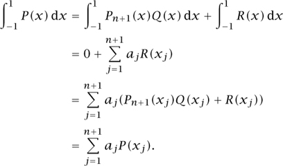
We have shown that the “quadrature formula” (9) is actually exact for all polynomials of degree at most 2n + 1, provided we choose the x_j to be the numbers suggested by Gauss. Unsurprisingly, this choice gives an extremely good way of estimating integrals numerically. “Gaussian quadrature” is one of the two main methods used to evaluate integrals on computers today.

We conclude with a brief look at a few other special functions.

Consider de Moivre’s formula

cos nθ + isin nθ = (cos θ + i sin θ)ⁿ.

Using the binomial expansion, we see that

and, taking real parts,

Since sin² θ = 1 – cos² θ, we have

where T_n is a polynomial of degree n called the nth Chebyshev polynomial. The Chebyshev polynomials play an important role in numerical analysis.

The next collection of functions requires us to calculate with infinite sums. Readers may treat our calculations as plausible or justify them rigorously according to taste. Observe first that

is well-defined for each real x that is not a multiple of π. Note also that h(x + π) = h(x) and = . Set f(x) = h(x) – cosec²(πx). By showing that there are constants K₁ and K₂ such that

and

for all , we deduce that there is a constant K such that |f(x)| < K for all 0 < x < π. Simple calculations show that

A single application of (10) shows that |f(x)| < K for all 0 < x < π, and repeated applications shows that f(x) = 0. Thus

for all real noninteger x.

If we seek analogues in the complex plane, we are led to functions of the type

Observe that, while the real function cosec² x satisfies cosec² (x + π) = cosec² (x) and is periodic with period π, the complex function F just defined satisfies

F(z + 1) = F(z),      F(z + i) = F(z)

and is doubly periodic with periods 1 and i. Functions like F are called elliptic functions and have a theory that parallels that Of the TRIGONOMETRIC FUNCTIONS [III.92].

The function is called the Gaussian or normal function and appears in probability and the study of diffusion processes (see [III.71 §5] and [IV.24]). The partial differential equation

with x corresponding to distance and t to time provides a reasonable model for diffusion. It is easy to check that ϕ(x, t) = ψ(x, t) = (Kt)^-1/2E(x(Kt)^-1/2) is a solution. By sketching a graph of ψ(x, t) as a function of x for various values of t, readers will see that ψ can be considered as the response to a disturbance at x = 0 when t = 0. By considering the behavior of ψ(x, t) as a function of t for a given value of x, they will see that “the effect at x of a disturbance at the origin becomes noticeable only after a time of the order x^1/2.” Living cells depend on diffusion processes and the result just given suggests (correctly) that such processes are very slow over long distances. It is plausible that this sets a limit on the size of a single cell: a large organism must be multi-celled.

Statisticians constantly use the related error function

There is a famous theorem of LIOUNILLE [VI.39] that shows that erf(x) cannot be expressed as a composition of elementary functions (such as quotients of polynomials, trigonometric functions, and EXPONENTIAL FUNCTIONS [III.2 5]).

We have been able to look at only a few properties of a few special functions in this article, but even this small sample shows how much interesting mathematics arises when we study one function or a class of particular functions rather than functions in general.