III.83 The Schrödinger Equation

Terence Tao

In mathematical physics, the Schrödinger equation (and the closely related Heisenberg equation) are the most fundamental equations in nonrelativistic quantum mechanics, playing the same role as Hamilton’s laws of motion (and the closely related Poisson equation) in nonrelativistic classical mechanics. (In relativistic quantum mechanics, the equations of quantum field theory take over the role of Heisenberg’s equation, while Schrödinger’s equation does not have a natural direct analogue.) In pure mathematics, the Schrödinger equation, together with its variants, is one of the basic equations studied in the field of PARTIAL DIFFERENTIAL EQUATIONS [IV.12], and has applications to geometry, to spectral and scattering theory, and to integrable systems.

The Schrödinger equation can be used to describe the quantum dynamics of many-particle systems under the influence of a variety of forces, but for simplicity let us consider just a single particle, of mass m > 0, moving about in n-dimensional space ⁿ subject to the influence of a potential, which we shall take to be a function V: ⁿ → . To avoid technicalities we shall assume that all the functions we discuss are smooth.

In classical mechanics, this particle would have a specific position q(t) ∈ ⁿ and a specific momentum p(t) ∈ ⁿ for each time t. (Eventually we shall observe the familiar law p(t) = mv(t), where v(t) = q'(t) is the velocity of the particle.) Thus, the state of this system at any given time t is described by the element (q(t), p(t)) of the space ⁿ × ⁿ, which is known as phase space. The energy of this state is described by the HAMILTONIAN FUNCTION [III.35] H: ⁿ × ⁿ → on phase space, defined in this case by

(Physically, the quantity represents kinetic energy, while V(q) represents potential energy.) The system then evolves according to Hamilton’s equations of motion:

where we keep in mind that p and q are vectors, so that these derivatives are GRADIENTS [I.3 § 5.3]. Hamilton’s equations of motion are valid for any classical system, but in our specific case of a particle in a “potential well,” they become

The first equation is asserting that p = mv, while the second equation is basically Newton’s second law of motion.

From (1) we can easily derive Poisson’s equation of motion

for any classical observable A: ⁿ × ⁿ → , where

is the Poisson bracket of H and A. Setting A = H, we have in particular the conservation-of-energy law:

for all t ∈ and some quantity E independent of t.

Now we analyze the quantum mechanical analogue of the above classical system. We need a small¹ parameter > 0, known as Planck’s constant. The state of the particle at a time t is no longer described by a single point (q(t), p(t)) in phase space, but is instead described by a wave function, which is a complex-valued function of position that evolves over time: that is, for each t we have a function ψ(t) from ⁿ to C. It is required to obey the normalization condition (ψ(t), ψ(t)) = 1, where (· , ·) denotes the inner product

Unlike a classical particle, a wave function ψ(t) does not necessarily have a specific position q(t). However, it does have an average position (q(t)), defined as

Here, we have written ψ(t, q) for the value of ψ(t) at the point q, and Q is the position operator, defined by (Qψ)(t, q) = qψ(t, q): that is, Q is the operator that multiplies pointwise by q. Similarly, while ψ does not have a specific momentum p(t), it does have an average momentum (p(t)), defined as

where the momentum opercitor P is defined by Planck’s law

Note that the vector (p (t)) is real-valued because all the components of P are SELF-ADJOINT [III.50 § 3.2]. More generally, given any quantum observable, by which we mean a self-adjoint OPERATOR [III.50] A acting on the space L²(ⁿ) of complex-valued square integrable functions, we can define the average value 〈A(t)〉 of A at time t by the formula

The analogue of Hamilton’s equations of motion (1) is now the time-dependent Schrödinger equation:

where H is now a quantum observable rather than a classical one. More precisely,

In other words, we have

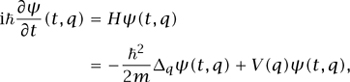
where

is the Laplacian of ψ. The analogue of Poisson’s equation of motion (3) is the Heisenberg equation

for any observable A, where [A, B] = AB - BA is the commutator or Lie bracket of A and B. (The quantity (i/) [A, B] is occasionally referred to as the quantum Poisson bracket of A and B.)

If the quantum state ψ oscillates in time according to the formula ψ (t, q) = for some real number E (known as the energy level or eigenvalue), then one has the time-independent Schrödinger equation:

(compare this with (4)). More generally, the important subject of spectral theory provides many links between the time-dependent equation (5) and the time-independent equation (7).

There are several strong analogies between the equations of classical mechanics and those of quantum mechanics. For instance, from (6) one has the equations

which should be compared with (2). Also, given any classical solution t (q(t), p(t)) to Hamilton’s equation of motion, one can construct a corresponding family of approximate solutions ψ(t) to Schrödinger’s equation, for instance by the formula²

where

is the classical action and ψ is any slowly varying function that is normalized in the sense that

One can verify that ψ solves (5) except for some errors that are small when is small. In physics, this fact is an example of the correspondence principle, which asserts that classical mechanics can be used to approximate quantum mechanics accurately if Planck’s constant is small and one is working at macroscopic scales (which is what allows us to use slowly varying functions ψ). In mathematics (and more precisely in the fields of microlocal analysis and semi-classical analysis), there are a number of formalizations of this principle that allow us to use knowledge about the behavior of Hamilton’s equations of motion in order to analyze the Schrödinger equation. For example, if the classical equations of motion have periodic solutions, then the Schrödinger equation often has nearly periodic solutions, whereas if the classical equations have very chaotic solutions, then the Schrödinger equation typically does as well (this phenomenon is known as quantum chaos or quantum ergodicity).

There are many aspects of the Schrödinger equation that are of interest. We mention just one of them here for illustration, namely that of scattering theory. If the potential function V decays sufficiently quickly at infinity, and k ∈ ⁿ is a nonzero frequency vector, then, setting the energy level as E = ²|k|²/2m, the time-independent Schrödinger equation Hψ = Eψ admits solutions ψ (q) that behave asymptotically (as |q| → ∞ as

for some canonical function f: S^n-1 × ⁿ →, C, which is known as the scattering amplitude function. This scattering amplitude depends (in a nonlinear fashion) on the potential V, and the map from V to f is known as the scattering transform. The scattering transform can be viewed as a nonlinear variant of THE FOURIER TRANSFORM [III.27]; it is connected to many areas of partial differential equations, such as the theory of integrable systems.

There are many generalizations and variants of the Schrödinger equation; one can generalize to many-particle systems, or add other forces such as magnetic fields or even nonlinear terms. One can also couple this equation to other physical equations such as MAXWELL’S EQUATIONS [IV.13 § 1.1] of electromagnetism, or replace the domain Rn by another space such as a torus, a discrete lattice, or a manifold. Alternatively, one could place some impenetrable obstacles in the domain (thus effectively removing those regions of space from the domain). The study of all of these variants leads to a vast and diverse field in both pure mathematics and in mathematical physics.

1. In many applications it is convenient to normalize (and m) to equal 1.

2. Intuitively, this function ψ (t, q) is localized in position near q(t) and localized in momentum near p(t), and is thus localized near (q(t), p(t)) in phase space. Such a localized function, exhibiting such “particle-like” behavior as having a reasonably well-defined position and velocity, is sometimes known as a “wave packet.” A typical solution of the Schrödinger equation does not behave like a wave packet, but can be decomposed as a superposition or linear combination of wave packets; such decompositions are a useful tool in analyzing general solutions of such equations.