FORMULATION OF THE BASIC MODEL

Our basic FFM expresses a firm's theoretical value as the sum of two level payment annuities reflecting a current earnings stream (the tangible value, TV) and a flow of net profits from expected future investments (the franchise value, FV):

TV is the economic book value associated with annual earnings derived from current businesses without the addition of new capital. In the FFM, we obtain a valuable simplification by viewing this earnings stream as a perpetual annuity, with annual payments E. This model annuity is presumed to have the same present value as the actual projected earnings stream. Any pattern of projected earnings can be replicated, in present value terms, by an appropriately chosen perpetual earnings stream.

In actuality, analysts use either trailing or forward-looking earnings projections. Realized earnings exhibit considerable year-to-year variability and optimistic earnings projections are often “front-loaded” with rapid growth in the early years and more stable and possibly declining earnings in later years. The opposite path is also possible: slow earnings growth projected in the early years and more rapid growth later.

If k is the risk-adjusted discount rate (usually taken as equivalent to the cost of equity capital), then³

The contribution of TV to the P/E ratio is obtained by dividing the above formula by E:

From the above formula, we see that P/E_TV depends only on the equity capitalization rate k. Since k depends on inflation, real rates and the equity risk premium, so does P/E_TV. These variables change over time, but they do so rather slowly. Consequently, we conclude that the P/E_TV is relatively stable.

In order to simplify the discussion in this chapter, we do not address the impact of inflation on both current and future earnings. It should be noted that a firm that can, even partially, “pass-through” inflation into earnings will be intrinsically more valuable and command a higher P/E than a firm that lacks the pricing power to pass-through inflation. More detailed discussion of the impact of inflation flow through on both TV and FV can be found in our earlier works.

The remaining source of value stems from future prospects to invest capital and obtain a premium return. Evaluations of such prospects require peering into a proverbial crystal ball in order to see the future. As such, these evaluations are subject to continual revision and have higher volatility.

There seems to be an almost congenital human need to view all growth as smooth and consistent, but any forced smoothing of growth prospects is likely to lead to a number of fundamental evaluation errors. In fact, investments in new businesses can only be established as opportunities arise in some irregular pattern over time. At the outset, each new business will require years of investment inflows, followed by subsequent years of (hopefully) positive returns. These returns will themselves vary from year to year. In the standard DDM, a fixed growth rate is chosen, and the size and timing of future projects are implicitly set by the level of earnings available for reinvestment.

In the FFM, we allow for a varying pattern of investments and returns. To do so, we model a project's investment and net return pattern as equivalent (in present value, PV) to a level annuity returning an appropriately chosen fixed rate R per dollar invested, year after year in perpetuity. The net new contribution to the firm's value is based on a fixed “franchise spread” (R – k) over the cost of capital earned on dollars invested. In the standard DDM, the return on new investments, R, is implicitly assumed to be the same as the return on the current book of business r. This rather restrictive return equality is not required implicitly or explicitly in the FFM.

Since investment dollars are contributed at various points in the future, we normalize each of those investment dollars by measuring them in terms of today's dollars (the PV). We then compute the sum of all PVs of investment dollars. This sum is the single dollar amount that, if invested today, would act as a surrogate for all future investments. The concept of the PV equivalence of the totality of future growth prospects has the virtue of considerable generality. No longer are we restricted to smooth compounded growth at some fixed rate. Virtually any future pattern of future opportunities—no matter how erratic—can be modeled through PV equivalence.

The PV of all growth opportunities will generally sum to a massive dollar value. To make this term intuitive and estimable, we represent it as a multiple, G, of current book value, B. That is,

or,

The totality of projected investments provides a perpetual stream of “net” profits with annual payments from the net spread earned by these investments:

FV is the present value of this perpetuity, which is calculated by dividing the above expression by k:

The contribution of FV to the P/E ratio is obtained by dividing the above formula by E, which can be represented as the product of the book value B and the current return on equity r:

We call the first factor on the right side of the above equation, the franchise factor (FF),

The above formulation allows for any pattern of new investments and returns over time including returns on new investments, R, that may be vastly different from the current return on equity, r. By focusing on the net PV of new investments, we avoid having to consider whether the financing is internal or external. While the classic DDM requires self-financing via earnings retention, there is no such limitation in the FFM.

The FFM formulation enables us to see through potentially unrealizable growth assumptions. In essence, the formulas above provide a “sanity check” against future expectations that are, in fact, unreasonable and virtually impossible to justify. The following examples illustrate how this works.

Imagine a growth firm that is presumed capable of providing a perpetual annual return on equity of 15%. The firm has a unique franchise that gives it substantial pricing power. By exercising this franchise, the firm is projected to be able to make new investments that will provide an even more attractive 18% perpetual annual return. This is surely would be considered a terrific firm if the cost of capital was only 9%! Under these assumptions,

and

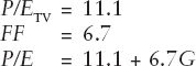
We leave G unspecified because it is the most difficult number to estimate but G will be the key to analyzing the P/E that the market currently assigns to this firm. For example, suppose the market multiple is 25×. In order to justify that P/E, G would have to be about 2.1.

The G factor is a bit mysterious, but worth exploring. G is the PV of all future invested dollars, expressed as a percentage of the firm's current economic book value. If we are thinking of a $100 million Firm V, then a G of 2.1 means that the PV of all future investments would be about $210 million. If this firm possesses new technology that the market is likely to embrace, $210 million of additional high return investments might be a modest, achievable requirement. Taken to the extreme, such a firm might have far greater future possibilities if, as expected, the new the new technology is widely embraced. In that case, the P/E might be far greater than 25×.

Now suppose Firm W is already a $10 billion dollar firm. Proportionately, Firm W must do exactly the same as Firm V to justify the same P/E. Firm W's challenge is really formidable—the required PV of all future investments is $21 billion!

The $21 billion figure is even more imposing when we realize that it represents the present value dollars of investments that earn and maintain, in perpetuity, a 9% average excess spread over the cost of capital. For example, if the firm made $3.2 billion in new investments every year for the next 10 years, the PV would be $21 billion but the total dollars invested would be $32 billion. Even for extraordinary firms with market sector dominance, finding such investments is not easy.

By using the FFM in this way, investors and analysts are positioned to ask the right questions. Does Firm W have the ability to find and execute $21 billion (in PV) of new investments that, on average, will provide an 18% return on equity in perpetuity? Does Firm V have that ability? The market, by assigning a P/E of 25× is saying the answer to both questions is a resounding “yes.”

This active questioning can be taken several steps further. What are the implications if the actual R is a little lower or higher than expected? How do the results change if the estimates of r are overly optimistic? What will happen if changing inflation expectations or changing equity risk premiums lead to changes in k?