6.6 Quantity Discount Models
In developing the EOQ model, we assumed that quantity discounts were not available. However, many companies do offer quantity discounts. If such a discount is possible, and all of the other EOQ assumptions are met, it is possible to find the quantity that minimizes the total inventory cost by using the EOQ model and making some adjustments.
When quantity discounts are available, the purchase cost or material cost becomes a relevant cost, as it changes based on the order quantity. The total relevant costs are as follows:
where
Since the holding cost per unit per year is based on the cost of the item, it is convenient to express this as
where
For a specific purchase cost (C), given the assumptions we have made, ordering the EOQ will minimize total inventory costs. However, in the discount situation, this quantity may not be large enough to qualify for the discount, so we must also consider ordering this minimum quantity for the discount. A typical quantity discount schedule is shown in Table 6.3.
As can be seen in the table, the normal cost for the item is $5. When 1,000 to 1,999 units are ordered at one time, the cost per unit drops to $4.80, and when the quantity ordered at one time is 2,000 or more units, the cost is $4.75 per unit. As always, management must decide when and how much to order. But with quantity discounts, how does the manager make these decisions?
As with other inventory models discussed so far, the overall objective will be to minimize the total cost. Because the unit cost for the third discount in Table 6.3 is lowest, you might be tempted to order 2,000 units or more to take advantage of the lower material cost. Placing an order for that quantity with the greatest discount cost, however, might not minimize the total inventory cost. As the discount quantity goes up, the material cost goes down, but the carrying cost increases because the orders are large. Thus, the major trade-off when considering quantity discounts is between the reduced material cost and the increased carrying cost.
Figure 6.6 provides a graphical representation of the total cost for this situation. Notice the cost curve drops considerably when the order quantity reaches the minimum for each discount. With the specific costs in this example, we see that the EOQ for the second price category is less than 1,000 units. Although the total cost for this EOQ is less than the total cost for the EOQ with the cost in category 1, the EOQ is not large enough to obtain this discount. Therefore, the lowest possible total cost for this discount price occurs at the minimum quantity required to obtain the discount The process for determining the minimum cost quantity in this situation is summarized in the following box.
Table 6.3 Quantity Discount Schedule
| DISCOUNT NUMBER | DISCOUNT QUANTITY | DISCOUNT (%) | DISCOUNT COST ($) |
|---|---|---|---|
| 1 | 0 to 999 | 0 | 5.00 |
| 2 | 1,000 to 1,999 | 4 | 4.80 |
| 3 | 2,000 and over | 5 | 4.75 |

Figure 6.6 Total Cost (TC) Curve for the Quantity Discount Model
Quantity Discount Model
For each discount price (C), compute
If EOQ < Minimum for discount, adjust the quantity to Q = Minimum for discount.
For each EOQ or adjusted Q, compute
Choose the lowest-cost quantity.
Brass Department Store Example
Let’s see how this procedure can be applied by showing an example. Brass Department Store stocks toy race cars. Recently, the store was given a quantity discount schedule for the cars; this quantity discount schedule is shown in Table 6.3. Thus, the normal cost for the toy race cars is $5. For orders between 1,000 and 1,999 units, the unit cost is $4.80, and for orders of 2,000 or more units, the unit cost is $4.75. Furthermore, the ordering cost is $49 per order, the annual demand is 5,000 race cars, and the inventory carrying charge as a percentage of cost, I, is 20% or 0.2. What order quantity will minimize the total inventory cost?
The first step is to compute EOQ for every discount in Table 6.3. This is done as follows:
The second step is to adjust those quantities that are below the allowable discount range. Since is between 0 and 999, it does not have to be adjusted. is below the allowable range of 1,000 to 1,999, and therefore it must be adjusted to 1,000 units. The same is true for it must be adjusted to 2,000 units. After this step, the following order quantities must be tested in the total cost equation:
The third step is to use Equation 6-14 to compute a total cost for each of the order quantities. This is accomplished with the aid of Table 6.4.
The fourth step is to select the order quantity with the lowest total cost. Looking at Table 6.4, you can see that an order quantity of 1,000 toy race cars minimizes the total cost. It should be recognized, however, that the total cost for ordering 2,000 cars is only slightly greater than the total cost for ordering 1,000 cars. Thus, if the third discount cost is lowered to $4.65, for example, this order quantity might be the one that minimizes the total inventory cost.
Using Excel QM for Quantity Discount Problems
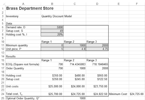
As seen in the previous analysis, the quantity discount model is more complex than the inventory models discussed so far in this chapter. Fortunately, we can use the computer to simplify the calculations. Program 6.3A shows the Excel formulas and input data needed for Excel QM for the Brass Department Store problem. Program 6.3B provides the solution to this problem, including adjusted order quantity and total cost for each price break.
Table 6.4 Total Cost Computations for Brass Department Store
| DISCOUNT NUMBER | UNIT PRICE (C) | ORDER QUANTITY (Q) | ANNUAL MATERIAL COST ($) = DC | ANNUAL ORDERING COST | ANNUAL CARRYING COST | TOTAL ($) |
|---|---|---|---|---|---|---|
| 1 | $5.00 | 700 | 25,000 | 350.00 | 350.00 | 25,700.00 |
| 2 | 4.80 | 1,000 | 24,000 | 245.00 | 480.00 | 24,725.00 |
| 3 | 4.75 | 2,000 | 23,750 | 122.50 | 950.00 | 24,822.50 |

Program 6.3A Excel QM Formulas and Input Data for the Brass Department Store Quantity Discount Problem