To use Excel 2016 for regression, enter the data in columns. Click the Data tab to access the data ribbon. Then select Data Analysis, as shown in Program 4.1A. If Data Analysis does not appear on the Data ribbon, the Excel add-in for this has not yet been activated. See Appendix F at the end of the book for instructions on how to activate this. Once this add-in is activated, it will remain on the Data ribbon for future use.

When the Data Analysis window opens, scroll down to and highlight Regression and click OK, as illustrated in Program 4.1A. The Regression window will open, as shown in Program 4.1B, and you can input the X and Y ranges. Check the Labels box because the cells in the first row of the X and Y ranges include the variable names. To have the output presented on this page rather than on a new worksheet, select Output Range and give a cell address for the start of the output. Click the OK button, and the output appears in the output range specified. Program 4.1C shows the intercept (2), slope (1.25), and other information that was previously calculated for the Triple A Construction example.

The sums of squares are shown in the column headed by SS. Another name for error is residual. In Excel, the sum of squares error is shown as the sum of squares residual. The values in this output are the same values shown in Table 4.3:

The coefficient of determination $\left(r^2\right)$ is shown to be 0.6944. The coefficient of correlation (r) is called Multiple R in the Excel output, and this is 0.8333.

Program 4.1B Data Input for Regression in Excel 2016

To use Excel QM for regression, from the Excel QM ribbon select the module by clicking Alphabetical - Forecasting - Multiple Regression, as shown in Program 4.2A. A window will open to allow you to specify the size of the problem, as shown in Program 4.2B. Enter a name or title for the problem, the number of past observations, and the number of independent (X) variables. For the Triple A Construction example, there are 6 past periods of data and 1 independent variable. When you click OK, a spreadsheet will appear for you to enter the X and Y data in the shaded area. The calculations are automatically performed, so there is nothing to do after entering the data. The results are seen in Program 4.2C.

Program 4.2C Input and Results for Regression in Excel QM

To develop a regression equation using QM for Windows for the Triple A Construction Company data, select the Forecasting module and select New. Then choose Least Squares—Simple and Multiple Regression, as illustrated in Program 4.3A. This opens the window shown in Program 4.3B. Enter the number of observations (6 in this example) and specify the number of independent variables (1 in this example). Left-click OK and a window opens allowing you to input the data, as shown in Program 4.3C. After entering the data, click Solve, and the forecasting results shown in Program 4.3D are displayed. The equation as well as other information is provided on this screen. Note the regression equation is displayed across two lines. Additional output, including the ANOVA table, is available by clicking the Window option on the toolbar.

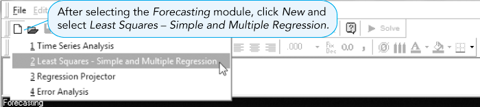
Program 4.3A QM for Windows Regression Option in Forecasting Module