 4.4 Assumptions of the Regression Model
by Trevor S. Hale, Michael E. Hanna, Ralph M. Stair, Barry Render
Quantitative Analysis for Management, 13/e
4.4 Assumptions of the Regression Model
by Trevor S. Hale, Michael E. Hanna, Ralph M. Stair, Barry Render
Quantitative Analysis for Management, 13/e
- Quantitative Analysis for Management
- About the Authors
- Brief Contents
- Contents
- Preface
- Chapter 1 Introduction to Quantitative Analysis
- Learning Objectives
- 1.1 What Is Quantitative Analysis?
- 1.2 Business Analytics
- 1.3 The Quantitative Analysis Approach
- 1.4 How to Develop a Quantitative Analysis Model
- 1.5 The Role of Computers and Spreadsheet Models in the Quantitative Analysis Approach
- 1.6 Possible Problems in the Quantitative Analysis Approach
- 1.7 Implementation—Not Just the Final StepImplementation—Not Just the Final Step
- Summary
- Glossary
- Key Equations
- Self-Test
- Discussion Questions and Problems
- Bibliography
- Chapter 2 Probability Concepts and Applications
- Learning Objectives
- 2.1 Fundamental Concepts
- 2.2 Revising Probabilities with Bayes’ TheoremRevising Probabilities with Bayes’ Theorem
- 2.3 Further Probability Revisions
- 2.4 Random Variables
- 2.5 Probability Distributions
- 2.6 The Binomial Distribution
- 2.7 The Normal Distribution
- 2.8 The F Distribution
- 2.9 The Exponential Distribution
- 2.10 The Poisson Distribution
- Summary
- Glossary
- Key Equations
- Solved Problems
- Self-Test
- Discussion Questions and Problems
- Bibliography
- Appendix 2.1: Derivation of Bayes’ TheoremDerivation of Bayes’ Theorem
- Chapter 3 Decision Analysis
- Learning Objectives
- 3.1 The Six Steps in Decision Making
- 3.2 Types of Decision-Making Environments
- 3.3 Decision Making Under Uncertainty
- 3.4 Decision Making Under Risk
- 3.5 Using Software for Payoff Table Problems
- 3.6 Decision Trees
- 3.7 How Probability Values Are Estimated by Bayesian Analysis
- 3.8 Utility Theory
- Summary
- Glossary
- Key Equations
- Solved Problems
- Self-Test
- Discussion Questions and Problems
- Bibliography
- Chapter 4 Regression Models
- Learning Objectives
- 4.1 Scatter Diagrams
- 4.2 Simple Linear Regression
- 4.3 Measuring the Fit of the Regression Model
- 4.4 Assumptions of the Regression Model
- 4.5 Testing the Model for Significance
- 4.6 Using Computer Software for Regression
- 4.7 Multiple Regression Analysis
- 4.8 Binary or Dummy Variables
- 4.9 Model Building
- 4.10 Nonlinear Regression
- 4.11 Cautions and Pitfalls in Regression Analysis
- Summary
- Glossary
- Key Equations
- Solved Problems
- Self-Test
- Discussion Questions and Problems
- Bibliography
- Appendix 4.1: Formulas for Regression Calculations
- Chapter 5 Forecasting
- Learning Objectives
- 5.1 Types of Forecasting Models
- 5.2 Components of a Time-Series
- 5.3 Measures of Forecast Accuracy
- 5.4 Forecasting Models—Random Variations OnlyForecasting Models—Random Variations Only
- 5.5 Forecasting Models—Trend and Random VariationsForecasting Models—Trend and Random Variations
- 5.6 Adjusting for Seasonal Variations
- 5.7 Forecasting Models—Trend, Seasonal, and Random VariationsForecasting Models—Trend, Seasonal, and Random Variations
- 5.8 Monitoring and Controlling Forecasts
- Summary
- Glossary
- Key Equations
- Solved Problems
- Self-Test
- Discussion Questions and Problems
- Chapter 6 Inventory Control Models
- Learning Objectives
- 6.1 Importance of Inventory Control
- 6.2 Inventory Decisions
- 6.3 Economic Order Quantity: Determining How Much to Order
- 6.4 Reorder Point: Determining When to Order
- 6.5 EOQ Without the Instantaneous Receipt Assumption
- 6.6 Quantity Discount Models
- 6.7 Use of Safety Stock
- 6.8 Single-Period Inventory Models
- 6.9 ABC Analysis
- 6.10 Dependent Demand: The Case for Material Requirements Planning
- 6.11 Just-In-Time Inventory Control
- 6.12 Enterprise Resource Planning
- Summary
- Glossary
- Key Equations
- Solved Problems
- Self-Test
- Discussion Questions and Problems
- Chapter 7 Linear Programming Models: Graphical and Computer Methods
- Learning Objectives
- 7.1 Requirements of a Linear Programming Problem
- 7.2 Formulating LP Problems
- 7.3 Graphical Solution to an LP Problem
- Corner Point Solution Method
- Slack and Surplus
- 7.4 Solving Flair Furniture’s LP Problem Using QM for Windows, Excel 2016, and Excel QMSolving Flair Furniture’s LP Problem Using QM for Windows, Excel 2016, and Excel QM
- 7.5 Solving Minimization Problems
- 7.6 Four Special Cases in LP
- 7.7 Sensitivity Analysis
- High Note Sound Company
- Changes in the Objective Function Coefficient
- QM for Windows and Changes in Objective Function Coefficients
- Excel Solver and Changes in Objective Function Coefficients
- Changes in the Technological Coefficients
- Changes in the Resources or Right-Hand-Side Values
- QM for Windows and Changes in Right-Hand-Side Values
- Excel Solver and Changes in Right-Hand-Side Values
- Summary
- Glossary
- Solved Problems
- Self-Test
- Discussion Questions and Problems
- Chapter 8 Linear Programming Applications
- Chapter 9 Transportation, Assignment, and Network Models
- Chapter10Integer Programming, Goal Programming, and Nonlinear Programming
- Chapter 11 Project Management
- Learning Objectives
- 11.1 PERT/CPM
- 11.2 PERT/Cost
- 11.3 Project Crashing
- 11.4 Other Topics in Project Management
- Summary
- Glossary
- Key Equations
- Solved Problems
- Self-Test
- Discussion Questions and Problems
- Bibliography
- Appendix 11.1: Project Management with QM for Windows
- Chapter 12 Waiting Lines and Queuing Theory Models
- Learning Objectives
- 12.1 Waiting Line Costs
- 12.2 Characteristics of a Queuing System
- 12.3 Single-Channel Queuing Model with Poisson Arrivals and Exponential Service Times (M/M /1)
- 12.4 Multichannel Queuing Model with Poisson Arrivals and Exponential Service Times (M ∕ ∕M ∕ ∕m)
- 12.5 Constant Service Time Model (M /D / 1)
- 12.6 Finite Population Model (M / M / 1 with Finite Source)
- 12.7 Some General Operating Characteristic Relationships
- 12.8 More Complex Queuing Models and the Use of Simulation
- Summary
- Glossary
- Key Equations
- Solved Problems
- Self-Test
- Discussion Questions and Problems
- Bibliography
- Appendix 12.1: Using QM for Windows
- Chapter 13 Simulation Modeling
- Learning Objectives
- 13.1 Advantages and Disadvantages of Simulation
- 13.2 Monte Carlo Simulation
- 13.3 Simulation and Inventory Analysis
- 13.4 Simulation of a Queuing Problem
- 13.5 Simulation Model for a Maintenance Policy
- Three Hills Power Company
- Column 1: Breakdown Number
- Column 2: Random Number for Breakdowns
- Column 3: Time Between Breakdowns
- Column 4: Time of Breakdown
- Column 5: Time Repairperson Is Free to Begin Repair
- Column 6: Random Number for Repair Time
- Column 7: Repair Time Required
- Column 8: Time Repair Ends
- Column 9: Number of Hours the Machine Is Down
- Cost Analysis of the Simulation
- Three Hills Power Company
- 13.6 Other Simulation Issues
- Summary
- Glossary
- Solved Problems
- Self-Test
- Discussion Questions and Problems
- Bibliography
- Chapter 14 Markov Analysis
- Learning Objectives
- 14.1 States and State Probabilities
- 14.2 Matrix of Transition Probabilities
- 14.3 Predicting Future Market Shares
- 14.4 Markov Analysis of Machine Operations
- 14.5 Equilibrium Conditions
- 14.6 Absorbing States and the Fundamental Matrix: Accounts Receivable Application
- Summary
- Glossary
- Key Equations
- Solved Problems
- Self-Test
- Discussion Questions and Problems
- Bibliography
- Appendix 14.1: Markov Analysis with QM for Windows
- Appendix 14.2: Markov Analysis with Excel
- Chapter 15 Statistical Quality Control
- Appendices
- Appendix B: Binomial Probabilities
- Appendix C: Values of e - λ for Use in the Poisson Distribution
- Appendix D: F Distribution Values
- Appendix E: Using POM-QM for Windows
- Appendix F: Using Excel QM and Excel Add-Ins
- Appendix G: Solutions to Selected Problems
- Appendix H: Solutions to Self-Tests
- Index
- Module 1 Analytic Hierarchy Process
- Module 2 Dynamic Programming
- Module 3 Decision Theory and the Normal Distribution
- Learning Objectives
- M3.1 Break-Even Analysis and the Normal Distribution
- M3.2 Expected Value of Perfect Information and the Normal Distribution
- Summary
- Glossary
- Key Equations
- Solved Problems
- Self-Test
- Discussion Questions and Problems
- Bibliography
- Appendix M3.1: Derivation of the Break-Even Point
- Appendix M3.2: Unit Normal Loss Integral
- Module 4 Game Theory
- Module 5Mathematical Tools: Determinants and Matrices
- Module 6 Calculus-Based Optimization
- Module 7 Linear Programming: The Simplex Method
- Module 8 Transportation, Assignment, and Network Algorithms
4.4 Assumptions of the Regression Model
If we can make certain assumptions about the errors in a regression model, we can perform statistical tests to determine if the model is useful. The following assumptions are made about the errors:
The errors are independent.
The errors are normally distributed.
The errors have a mean of zero.
The errors have a constant variance (regardless of the value of X).
It is possible to check the data to see if these assumptions are met. Often a plot of the residuals will highlight any glaring violations of the assumptions. When the errors (residuals) are plotted against the independent variable, the pattern should appear random.
Figure 4.4 presents some typical error patterns, with Figure 4.4A displaying a pattern that is expected when the assumptions are met and the model is appropriate. The errors are random and no discernible pattern is present. Figure 4.4B demonstrates an error pattern in which the errors increase as X increases, violating the constant variance assumption. Figure 4.4C shows errors consistently increasing at first and then consistently decreasing. A pattern such as this would indicate that the model is not linear and some other form (perhaps quadratic) should be used. In general, patterns in the plot of the errors indicate problems with the assumptions or the model specification.

Figure 4.4A Pattern of Errors Indicating Randomness

Figure 4.4B Nonconstant Error Variance
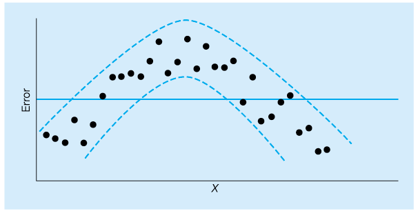
Figure 4.4C Pattern of Errors Indicating Relationship Is Not Linear
Estimating the Variance
While the errors are assumed to have constant variance
where
In the Triple A Construction example,
From this, we can estimate the standard deviation as
This is called the standard error of the estimate or the standard deviation of the regression. In this example,
This is used in many of the statistical tests about the model. It is also used to find interval estimates for both Y and regression coefficients.2
-
No Comment