
3.6 Decision Trees
Any problem that can be presented in a decision table can also be graphically illustrated in a decision tree. All decision trees are similar in that they contain decision nodes or decision points and state-of-nature nodes or state-of-nature points:
A decision node from which one of several alternatives may be chosen
A state-of-nature node out of which one state of nature will occur
In drawing the tree, we begin at the left and move to the right. Thus, the tree presents the decisions and outcomes in sequential order. Lines or branches from the squares (decision nodes) represent alternatives, and branches from the circles represent the states of nature. Figure 3.2 gives the basic decision tree for the Thompson Lumber example. First, John decides whether to construct a large plant, a small plant, or no plant. Then, once that decision is made, the possible states of nature or outcomes (favorable or unfavorable market) will occur. The next step is to put the payoffs and probabilities on the tree and begin the analysis.
Analyzing problems with decision trees involves five steps:
Five Steps of Decision Tree Analysis
Define the problem.
Structure or draw the decision tree.
Assign probabilities to the states of nature.
Estimate payoffs for each possible combination of alternatives and states of nature.
Solve the problem by computing EMVs for each state-of-nature node. This is done by working backward, that is, starting at the right of the tree and working back to decision nodes on the left. Also, at each decision node, the alternative with the best EMV is selected.
The final decision tree with the payoffs and probabilities for John Thompson’s decision situation is shown in Figure 3.3. Note that the payoffs are placed at the right side of each of the tree’s branches. The probabilities are shown in parentheses next to each state of nature. Beginning with the payoffs on the right of the figure, the EMVs for each state-of-nature node are then calculated and placed by their respective nodes. The EMV of the first node is $10,000. This represents the branch from the decision node to construct a large plant. The EMV for node 2, to construct a small plant, is $40,000. Building no plant or doing nothing has, of course, a payoff of $0. The branch leaving the decision node leading to the state-of-nature node with the highest EMV should be chosen. In Thompson’s case, a small plant should be built.
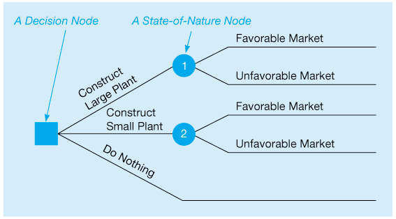
Figure 3.2 Thompson’s Decision Tree

Figure 3.3 Completed and Solved Decision Tree for Thompson Lumber
A More Complex Decision for Thompson Lumber—Sample Information
When sequential decisions need to be made, decision trees are much more powerful tools than decision tables. Let’s say that John Thompson has two decisions to make, with the second decision dependent on the outcome of the first. Before deciding about building a new plant, John has the option of conducting his own marketing research survey, at a cost of $10,000. The information from his survey could help him decide whether to construct a large plant or a small plant or not to build at all. John recognizes that such a market survey will not provide him with perfect information, but it may help quite a bit nevertheless.
John’s new decision tree is represented in Figure 3.4. Let’s take a careful look at this more complex tree. Note that all possible outcomes and alternatives are included in their logical sequence. This is one of the strengths of using decision trees in making decisions. The user is forced to examine all possible outcomes, including unfavorable ones. He or she is also forced to make decisions in a logical, sequential manner.
Examining the tree, we see that Thompson’s first decision point is whether to conduct the $10,000 market survey. If he chooses not to do the study (the lower part of the tree), he can construct a large plant, a small plant, or no plant. This is John’s second decision point. The market will be either favorable (0.50 probability) or unfavorable (also 0.50 probability) if he builds. The payoffs for each of the possible consequences are listed along the right side. As a matter of fact, the lower portion of John’s tree is identical to the simpler decision tree shown in Figure 3.3. Why is this so?
The upper part of Figure 3.4 reflects the decision to conduct the market survey. State-of- nature node 1 has two branches. There is a 45% chance that the survey results will indicate a favorable market for storage sheds. We also note that the probability is 0.55 that the survey results will be negative. The derivation of this probability will be discussed in the next section.
The rest of the probabilities shown in parentheses in Figure 3.4 are all conditional probabilities or posterior probabilities (these probabilities will also be discussed in the next section). For example, 0.78 is the probability of a favorable market for the sheds given a favorable result from the market survey. Of course, you would expect to find a high probability of a favorable market given that the research indicated that the market was good. Don’t forget, though, there is a chance that John’s $10,000 market survey didn’t result in perfect or even reliable information. Any market research study is subject to error. In this case, there is a 22% chance that the market for sheds will be unfavorable given that the survey results are positive.
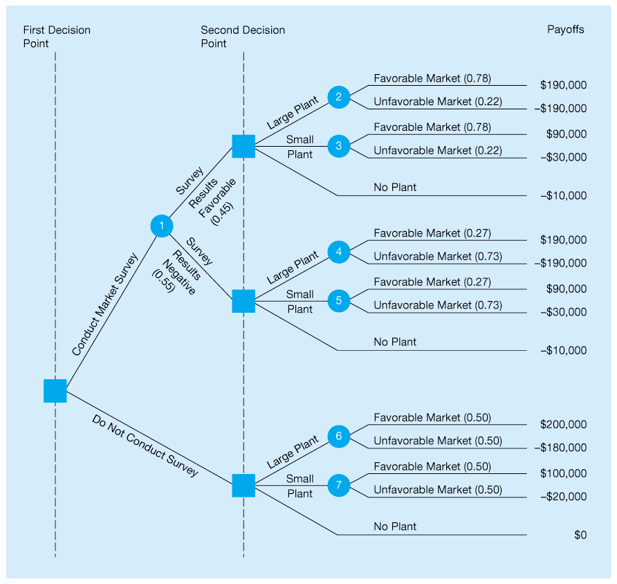
Figure 3.4 Larger Decision Tree with Payoffs and Probabilities for Thompson Lumber
We note that there is a 27% chance that the market for sheds will be favorable given that John’s survey results are negative. The probability is much higher, 0.73, that the market will actually be unfavorable given that the survey was negative.
Finally, when we look to the payoff column in Figure 3.4, we see that $10,000, the cost of the marketing study, had to be subtracted from each of the top 10 tree branches. Thus, a large plant with a favorable market would normally net a $200,000 profit. But because the market study was conducted, this figure is reduced by $10,000 to $190,000. In the unfavorable case, the loss of $180,000 would increase to a greater loss of $190,000. Similarly, conducting the survey and building no plant now results in a payoff.
With all probabilities and payoffs specified, we can start calculating the EMV at each state-of-nature node. We begin at the end, or right side of the decision tree, and work back toward the origin. When we finish, the best decision will be known.
Given favorable survey results,
The EMV of no plant in this case is $10,000. Thus, if the survey results are favorable, a large plant should be built. Note that we bring the expected value of this decision ($106,400) to the decision node to indicate that if the survey results are positive, our expected value will be $106,400. This is shown in Figure 3.5.
Given negative survey results,

Figure 3.5 Thompson’s Decision Tree with EMVs Shown
The EMV of no plant is again for this branch. Thus, given a negative survey result, John should build a small plant with an expected value of $2,400, and this figure is indicated at the decision node.
Continuing on the upper part of the tree and moving backward, we compute the expected value of conducting the market survey:
If the market survey is not conducted,
The EMV of no plant is $0.
Thus, building a small plant is the best choice, given that the marketing research is not performed, as we saw earlier.
We move back to the first decision node and choose the best alternative. The EMV of conducting the survey is $49,200, versus an EMV of $40,000 for not conducting the study, so the best choice is to seek marketing information. If the survey results are favorable, John should construct a large plant, but if the research is negative, John should construct a small plant.
In Figure 3.5, these expected values are placed on the decision tree. Notice on the tree that a pair of slash lines / / through a decision branch indicates that particular alternative is dropped from further consideration. This is because its EMV is lower than the EMV for the best alternative. After you have solved several decision tree problems, you may find it easier to do all of your computations on the tree diagram.
Expected Value of Sample Information
With the market survey he intends to conduct, John Thompson knows that his best decision will be to build a large plant if the survey is favorable or a small plant if the survey results are negative. But John also realizes that conducting the market research is not free. He would like to know what the actual value of doing a survey is. One way of measuring the value of market information is to compute the expected value of sample information (EVSI), which is the increase in expected value resulting from the sample information.
The expected value with sample information (EV with SI) is found from the decision tree, and the cost of the sample information is added to this, since this was subtracted from all the payoffs before the EV with SI was calculated. The expected value without sample information (EV without SI) is then subtracted from this to find the value of the sample information.
where
In John’s case, his EMV would be $59,200 if he hadn’t already subtracted the $10,000 study cost from each payoff. (Do you see why this is so? If not, add $10,000 back into each payoff, as in the original Thompson problem, and recompute the EMV of conducting the market study.) From the lower branch of Figure 3.5, we see that the EMV of not gathering the sample information is $40,000. Thus,
This means that John could have paid up to $19,200 for a market study and still come out ahead. Since it costs only $10,000, the survey is indeed worthwhile.
Efficiency of Sample Information
There may be many types of sample information available to a decision maker. In developing a new product, information could be obtained from a survey, from a focus group, from other market research techniques, or from actual use of a test market to see how sales will be. While none of these sources of information are perfect, they can be evaluated by comparing the EVSI with the EVPI. If the sample information was perfect, then the efficiency would be 100%. The efficiency of sample information is
In the Thompson Lumber example,
Thus, the market survey is only 32% as efficient as perfect information.
Sensitivity Analysis
As with payoff tables, sensitivity analysis can be applied to decision trees as well. The overall approach is the same. Consider the decision tree for the expanded Thompson Lumber problem shown in Figure 3.5. How sensitive is our decision (to conduct the marketing survey) to the probability of favorable survey results?
Let p be the probability of favorable survey results. Then is the probability of negative survey results. Given this information, we can develop an expression for the EMV of conducting the survey, which is node 1:
We are indifferent when the EMV of conducting the marketing survey, node 1, is the same as the EMV of not conducting the survey, which is $40,000. We can find the indifference point by equating EMV(node 1) to $40,000:
As long as the probability of favorable survey results, p, is greater than 0.36, our decision will stay the same. When p is less than 0.36, our decision will be not to conduct the survey.
We could also perform sensitivity analysis for other problem parameters. For example, we could find how sensitive our decision is to the probability of a favorable market given favorable survey results. At this time, this probability is 0.78. If this value goes up, the large plant becomes more attractive. In this case, our decision would not change. What happens when this probability goes down? The analysis becomes more complex. As the probability of a favorable market (given favorable survey) result goes down, the small plant becomes more attractive. At some point, the small plant will result in a higher EMV (given favorable survey results) than the large plant. This, however, does not conclude our analysis. As the probability of a favorable market (given favorable survey results) continues to fall, there will be a point where not conducting the survey, with an EMV of $40,000, will be more attractive than conducting the marketing survey. We leave the actual calculations to you. It is important to note that sensitivity analysis should consider all possible consequences.