
M7.4 Solving Minimization Problems
Now that we have discussed how to deal with objective functions and constraints associated with minimization problems, let’s see how to use the simplex method to solve a typical problem.
The Muddy River Chemical Corporation Example
The Muddy River Chemical Corporation must produce exactly 1,000 pounds of a special mixture of phosphate and potassium for a customer. Phosphate costs $5 per pound and potassium costs $6 per pound. No more than 300 pounds of phosphate can be used, and at least 150 pounds of potassium must be used. The problem is to determine the least-cost blend of the two ingredients.
This problem may be restated mathematically as
where
Note that there are three constraints, not counting the nonnegativity constraints: the first is an equality, the second is a less-than-or-equal-to constraint, and the third is a greater-than-or-equal-to constraint.
Graphical Analysis
To have a better understanding of the problem, a brief graphical analysis may prove useful. There are only two decision variables, X1
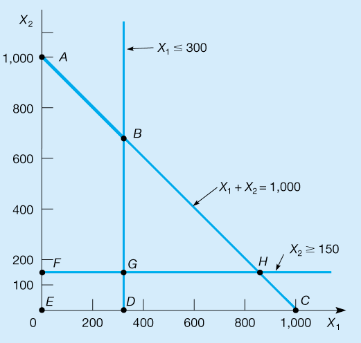
Figure M7.3 Muddy River Chemical Corporation’s Feasible Region Graph
You don’t need the simplex method to solve the Muddy River Chemical problem, of course. But we can guarantee you that few problems will be this simple. In general, you can expect to see several variables and many constraints. The purpose of this section is to illustrate the straightforward application of the simplex method to minimization problems. When the simplex procedure is used to solve this, it will methodically move from corner point to corner point until the optimal solution is reached. In Figure M7.3, the simplex method will begin at point E, then move to point F, then to point G, and finally to point B, which is the optimal solution.
Converting the Constraints and Objective Function
The first step is to apply what we learned in the preceding section to convert the constraints and objective function into the proper form for the simplex method. The equality constraint, X1+X2=1,000,
Table M7.7 Initial Simplex Tableau for the Muddy River Chemical Corporation Problem

The second constraint, X1≤300,
The last constraint is X2≥150,
Finally, the objective function, cost=$5X1+$6X2,
The complete set of constraints can now be expressed as follows:
Rules of the Simplex Method for Minimization Problems
Minimization problems are quite similar to the maximization problems tackled earlier in this module. The significant difference involves the Cj−Zj
Stpng for Simplex Minimization Problems
Choose the variable with a negative Cj−Zj
Cj−Zj that indicates the largest decrease in cost to enter the solution. The corresponding column is the pivot column.Determine the row to be replaced by selecting the one with the smallest (nonnegative) ratio of quantity to pivot column substitution rate. This is the pivot row.
Calculate new values for the pivot row.
Calculate new values for the other rows.
Calculate the Zj
Zj and Cj−ZjCj−Zj values for this tableau. If there are any Cj−ZjCj−Zj numbers less than 0, return to step 1.
First Simplex Tableau for the Muddy River Chemical Corporation Problem
Now we solve Muddy River Chemical Corporation’s LP formulation using the simplex method. The initial tableau is set up just as in the earlier maximization example. Its first three rows are shown in the accompanying table. We note the presence of the $M costs associated with artificial variables A1
| Cj | SOLUTION MIX | X1 | X2 | S1 | S2 | A1 | A2 | QUANTITY |
|---|---|---|---|---|---|---|---|---|
| $M | A1 |
1 | 1 | 0 | 0 | 1 | 0 | 1,000 |
| $0 | S1 |
1 | 0 | 1 | 0 | 0 | 0 | 300 |
| $M | A2 |
0 | 1 | 0 | 21 |
0 | 1 | 150 |
The numbers in the Zj
The Cj−Zj
| COLUMN | ||||||
|---|---|---|---|---|---|---|
| X1 | X2 | S1 | S2 | A1 | A2 | |
| Cj |
$5 | $6 | $0 | $0 | $M | $M |
| Zj |
$M | $2M | $0 | −$M |
$M | $M |
| Cj−Zj |
−$M+$5 |
−$2M+$6 |
$0 | $M | $0 | $0 |
This initial solution was obtained by letting each of the variables X1, X2,
An extremely high cost, $1,150M from Table M7.7, is associated with this answer. We know that this can be reduced significantly and now move on to the solution procedures.
Developing a Second Tableau
In the Cj−Zj
Which variable will leave the solution to make room for the new variable, X2?
Hence, the pivot row is the A2
The entering row for the next simplex tableau is found by dividing each element in the pivot row by the pivot number, 1. This leaves the old pivot row unchanged, except that it now represents the solution variable X2.

The Zj
| COLUMN | ||||||
|---|---|---|---|---|---|---|
| X1 | X2 | S1 | S2 | A1 | A2 | |
| Cj |
$5 | $6 | $0 | $0 | $M | $M |
| Zj |
$M | $6 | $0 | $ M−6 |
$M | −$ M+6 |
| Cj−Zj |
−$ M+5 |
$0 | $0 | −$ M+6 |
$0 | $ −M−6 |
All of these computational results are presented in Table M7.8.
Table M7.8 Second Simplex Tableau for the Muddy River Chemical Corporation Problem

The solution at the end of the second tableau (point F in Figure M7.3) is A1=850,
Developing a Third Tableau
The new pivot column is the X1
Hence, variable S1
To replace the pivot row, we divide each number in the S1
Table M7.9 Third Simplex Tableau for the Muddy River Chemical Corporation Problem


The Zj
| COLUMN | ||||||
|---|---|---|---|---|---|---|
| X1 | X2 | S1 | S2 | A1 | A2 | |
| Cj for column | $5 | $6 | $0 | $0 | $M | $M |
| Zj for column | $5 | $6 | −$ M+5 | $ M−6 | $M | −$ M+6 |
| Cj−Zj for column | $0 | $0 | $ M−5 | −$ M+6 | $0 | $ 2M−6 |
The solution at the end of the three iterations (point G in Figure M7.3) is still not optimal because the S2 column contains a Cj−Zj value that is negative. Note that the current total cost is nonetheless lower than at the end of the second tableau, which in turn is lower than the initial solution cost. We are headed in the right direction but have one more tableau to go!
Fourth Tableau for the Muddy River Chemical Corporation Problem
The pivot column is now the S2 column. The ratios that determine the row and variable to be replaced are computed as follows:
Each number in the pivot row is divided by the pivot number (again 1, by coincidence). The other two rows are computed as follows and are shown in Table M7.10:

COLUMN
X1
X2
S1
S2
A1
A2
Cj for column
$5
$6
$0
$0
$M
$M
Zj for column
$5
$6
−$ 1
$0
$6
$0
Cj−Zj for column
$0
$0
$1
$0
$M $M−6
$M
Table M7.10 Fourth and Optimal Solution to the Muddy River Chemical Corporation Problem

On examining the Cj−Zj row in Table M7.10, only positive or 0 values are found. The fourth tableau therefore contains the optimum solution. That solution is X1=300, X2=700, and S2=550. The artificial variables are both equal to 0, as is S1. Translated into management terms, the chemical company’s decision should be to blend 300 pounds of phosphate (X1) with 700 pounds of potassium (X2). This provides a surplus (S2) of 550 pounds of potassium more than required by the constraint X2≥150. The cost of this solution is $5,700. If you look back to Figure M7.3, you can see that this is identical to the answer found by the graphical approach.
Although small problems such as this can be solved graphically, more realistic product blending problems demand use of the simplex method, usually in computerized form.
Review of Procedures for Solving LP Minimization Problems
Just as we summarized the stpng for solving LP maximization problems with the simplex method, let us do so for minimization problems here:
Formulate the LP problem’s objective function and constraints.
Include slack variables in each less-than-or-equal-to constraint, artificial variables in each equality constraint, and both surplus and artificial variables in each greater-than-or-equal-to constraint. Then add all of these variables to the problem’s objective function.
Develop an initial simplex tableau with artificial and slack variables in the basis and the other variables set equal to 0. Compute the Zj and Cj−Zj values for this tableau.
Follow these five stpng until an optimal solution has been reached:
Choose the variable with the negative Cj−Zj indicating the greatest improvement to enter the solution. This is the pivot column.
Determine the row to be replaced by selecting the one with the smallest (nonnegative) ratio of quantity to pivot column substitution rate. This is the pivot row.
Calculate the new values for the pivot row.
Calculate the new values for the other row(s).
Calculate the Zj and Cj−Zj values for the tableau. If there are any Cj−Zj numbers less than 0, return to step 1. If there are no Cj−Zj numbers that are less than 0, an optimal solution has been reached.
M7.5 Special Cases
In Chapter 7, we addressed some special cases that may arise when solving LP problems graphically (see Section 7.6). Here we describe these cases again, this time as they refer to the simplex method.
Infeasibility
Infeasibility, you may recall, comes about when there is no solution that satisfies all of the problem’s constraints. In the simplex method, an infeasible solution is indicated by looking at the final tableau. In it, all Cj−Zj row entries will be of the proper sign to imply optimality, but an artificial variable (A1) will still be in the solution mix.
Table M7.11 illustrates the final simplex tableau for a hypothetical minimization type of LP problem. The table provides an example of an improperly formulated problem, probably containing conflicting constraints. No feasible solution is possible because an artificial variable, A2, remains in the solution mix, even though all Cj−Zj entries are positive or 0 (the criterion for an optimal solution in a minimization case).
Table M7.11 Illustration of Infeasibility

Unbounded Solutions
Unboundedness describes linear programs that do not have finite solutions. It occurs in maximization problems, for example, when a solution variable can be made infinitely large without violating a constraint. In the simplex method, the condition of unboundedness will be discovered prior to reaching the final tableau. We will note the problem when trying to decide which variable to remove from the solution mix. As seen earlier in this module, the procedure is to divide each quantity column number by the corresponding pivot column number. The row with the smallest positive ratio is replaced. But if all the ratios turn out to be negative or undefined, it indicates that the problem is unbounded.
Table M7.12 illustrates the second tableau calculated for a particular LP maximization problem by the simplex method. It also points to the condition of unboundedness. The solution is not optimal because not all Cj−Zj entries are 0 or negative, as required in a maximization problem. The next variable to enter the solution should be X1. To determine which variable will leave the solution, we examine the ratios of the quantity column numbers to their corresponding numbers in the X1, or pivot, column:

Since both pivot column numbers are negative, an unbounded solution is indicated.
Table M7.12 Problem with an Unbounded Solution

Degeneracy
Degeneracy is another situation that can occur when solving an LP problem using the simplex method. It develops when three (or more) constraints pass through a single point. For example, suppose a problem has only these three constraints X1≤10, X2≤10, and X1+X2<20. All three constraint lines will pass through the point (10, 10). Degeneracy is first recognized when the ratio calculations are made. If there is a tie for the smallest ratio, this is a signal that degeneracy exists. As a result of this, when the next tableau is developed, one of the variables in the solution mix will have a value of zero.
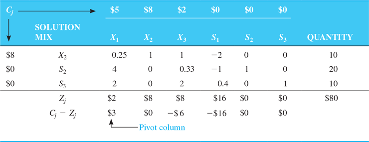
Table M7.13 provides an example of a degenerate problem. At this iteration of the given maximization LP problem, the next variable to enter the solution will be X1, since it has the only positive Cj−Zj number. The ratios are computed as follows:
Theoretically, degeneracy could lead to a situation known as cycling, in which the simplex algorithm alternates back and forth between the same nonoptimal solutions; that is, it puts a new variable in, then takes it out in the next tableau, then puts it back in, and so on. One simple way of dealing with the issue is to select either row (S2 or S3, in this case) arbitrarily. If we are unlucky and cycling does occur, we simply go back and select the other row.
Table M7.13 Problem Illustrating Degeneracy
More Than One Optimal Solution
Multiple, or alternate, optimal solutions can be spotted when the simplex method is being used by looking at the final tableau. If the Cj−Zj value is equal to 0 for a variable that is not in the solution mix, more than one optimal solution exists.
Let’s take Table M7.14 as an example. Here is the last tableau of a maximization problem; each entry in the Cj−Zj row is 0 or negative, indicating that an optimal solution has been reached. That solution is read as X2=6, S2=3, and profit=$12. Note, however, that variable X1 can be brought into the solution mix without increasing or decreasing profit. The new solution, with X1 in the basis, would become X1 = 3 and X2=1.5, with profit still at $12. Can you modify Table M7.14 to prove this?
Table M7.14 Problem with Alternate Optimal Solutions

M7.6 Sensitivity Analysis with the Simplex Tableau
In Chapter 7, we introduce the topic of sensitivity analysis as it applies to LP problems that we have solved graphically. This valuable concept shows how the optimal solution and the value of its objective function change given changes in various inputs to the problem. Graphical analysis is useful in understanding intuitively and visually how feasible regions and the slopes of objective functions can change as model coefficients change. Computer programs handling LP problems of all sizes provide sensitivity analysis as an important output feature. Those programs use the information provided in the final simplex tableau to compute ranges for the objective function coefficients and ranges for the RHS values. They also provide shadow prices, a concept that we introduce in this section.
High Note Sound Company Revisited
In Chapter 7, we use the High Note Sound Company to illustrate sensitivity analysis graphically. High Note is a firm that makes quality speakers (called X1) and stereo receivers (called X2). Its LP formulation is repeated here:
High Note’s graphical solution is repeated in Figure M7.4.

Figure M7.4 High Note Sound Company Graphical Solution
Changes in the Objective Function Coefficients
In Chapter 7, we saw how to use graphical LP to examine the objective function coefficients.
A second way of illustrating the sensitivity analysis of objective function coefficients is to consider the problem’s final simplex tableau. For the High Note Sound Company, this tableau is shown in Table M7.15. The optimal solution is seen to be as follows:

Basic variables (those in the solution mix) and nonbasic variables (those set equal to 0) must be handled differently using sensitivity analysis. Let us first consider the case of a nonbasic variable.
Table M7.15 Optimal Solution by the Simplex Method

Nonbasic Objective Function Coefficient
Our goal here is to find out how sensitive the problem’s optimal solution is to changes in the contribution rates of variables not currently in the basis (X1 and S1). Just how much would the objective function coefficients have to change before X1 or S1 would enter the solution mix and replace one of the basic variables?
The answer lies in the Cj−Zj row of the final simplex tableau (as in Table M7.15). Since this is a maximization problem, the basis will not change unless the Cj−Zj value of one of the nonbasic variables becomes positive. That is, the current solution will be optimal as long as all numbers in the bottom row are less than or equal to 0. It will not be optimal if X1’s Cj−Zj value is positive or if S1’s Cj−Zj value is greater than 0. Therefore, the values of Cj for X1 and S1 that do not bring about any change in the optimal solution are given by
This is the same as writing
Since X1’s Cj value is $50 and its Zj value is $60, the current solution is optimal as long as the profit per speaker does not exceed $60 or, correspondingly, does not increase by more than $10. Similarly, the contribution rate per unit of S1 (or per hour of electrician’s time) may increase from $0 up to $30 without changing the current solution mix.
In both cases, when you are maximizing an objective function, you may increase the value of Cj up to the value of Zj. You may also decrease the value of Cj for a nonbasic variable to negative infinity (−∞) without affecting the solution. This range of Cj values is called the range of insignificance for nonbasic variables.
Basic Objective Function Coefficient
Sensitivity analysis on objective function coefficients of variables that are in the basis or solution mix is slightly more complex. We saw that a change in the objective function coefficient for a nonbasic variable affects only the Cj−Zj value for that variable. But a change in the profit or cost of a basic variable can affect the Cj−Zj values of all nonbasic variables because this Cj is not only in the Cj row but also in the Cj column. This then impacts the Zj row.
Let us consider changing the profit contribution of stereo receivers in the High Note Sound Company problem. Currently, the objective function coefficient is $120. The change in this value can be denoted by the Greek capital letter delta (Δ). We rework the final simplex tableau (first shown in Table M7.15) and see our results in Table M7.16.
Table M7.16 Change in the Profit Contribution of Stereo Receivers

Notice the new Cj−Zj values for nonbasic variables X1 and S1. These were determined in exactly the same way as we did earlier in this module. But wherever the Cj value for X2 of $120 was seen in Table M7.15, a new value of $120+Δ is used in Table M7.16.
Once again, we recognize that the current optimal solution will change only if one or more of the Cj−Zj row values becomes greater than 0. The question is, how may the value of Δ vary so that all Cj−Zj entries remain negative? To find out, we solve for Δ in each column.
From the X1 column:
This inequality means that the optimal solution will not change unless X2’s profit coefficient decreases by at least $20, which is a change of Δ=−$20. Hence, variable X1 will not enter the basis unless the profit per stereo receiver drops from $120 to $100 or less. This, interestingly, is exactly what we noticed graphically in Chapter 7. When the profit per stereo receiver dropped to $80, the optimal solution changed from corner point a to corner point b.
Now we examine the S1 column:
This inequality implies that S1 is less sensitive to change than X1. S1 will not enter the basis unless the profit per unit of X2 drops from $120 all the way down to $0.
Since the first inequality is more binding, we can say that the range of optimality for X2’s profit coefficient is
As long as the profit per stereo receiver is greater than or equal to $100, the current production mix of X2=20 receivers and X1=0 speakers will be optimal.
In analyzing larger problems, we would use this procedure to test for the range of optimality of every real decision variable in the final solution mix. The procedure helps us avoid the time-consuming process of reformulating and resolving the entire LP problem each time a small change occurs. Within the bounds set, changes in profit coefficients would not force a firm to alter its product mix decision or change the number of units produced. Overall profits, of course, will change if a profit coefficient increases or decreases, but such computations are quick and easy to perform.
Changes in Resources or RHS Values
Making changes in the RHS values (the resources of electricians’ and audio technicians’ time) results in changes in the feasible region and often the optimal solution.
Shadow Prices
This leads us to the important subject of shadow prices. Exactly how much should a firm be willing to pay to make additional resources available? Is one more hour of machine time worth $1 or $5 or $20? Is it worthwhile to pay workers an overtime rate to stay one extra hour each night to increase production output? Valuable management information could be provided if the worth of additional resources were known.
Fortunately, this information is available to us by looking at the final simplex tableau of an LP problem. An important property of the Cj−Zj row is that the negatives of the numbers in its slack variable (Si) columns provide us with what we call shadow prices. A shadow price is the change in value of the objective function from an increase of one unit of a scarce resource (e.g., when one more hour of machine time or labor time or other resource is made available).
The final simplex tableau for the High Note Sound Company problem is repeated as Table M7.17 (it was first shown as Table M7.15). The tableau indicates that the optimal solution is X1=0, X2=20, S1=0, and S2=40 and that profit=$ 2,400. Recall that S1 represents slack availability of the electricians’ resource and S2 the unused time in the audio technicians’ department.
Table M7.17 Final Tableau for the High Note Sound Company

The firm is considering hiring an extra electrician on a part-time basis. Let’s say that it will cost $22 per hour in wages and benefits to bring the part-timer on board. Should the firm do this? The answer is yes: the shadow price of the electrician time resource is $30. Thus, the firm will net $8 (=$30−$22) for every hour the new worker helps in the production process.
Should High Note also hire a part-time audio technician at a rate of $14 per hour? The answer is no: the shadow price is $0, implying no increase in the objective function by making more of this second resource available. Why? Because not all of the resource is currently being used—40 hours are still available. It would hardly pay to buy more of the resource.
Right-Hand-Side Ranging
Obviously, we can’t add an unlimited number of units of resource without eventually violating one of the problem’s constraints. When we understand and compute the shadow price for an additional hour of electricians’ time ($30), we will want to determine how many hours we can actually use to increase profits. Should the new resource be added 1 hour, 2 hours, or 200 hours per week? In LP terms, this process involves finding the range over which shadow prices will stay valid. Right-hand-side ranging tells us the number of hours High Note can add or remove from the electrician department and still have a shadow price of $30.
Ranging is simple in that it resembles the simplex process we used earlier in this module to find the minimum ratio for a new variable. The S1 column and quantity column from Table M7.17 are repeated in the following table; the ratios, both positive and negative, are also shown:
| Quantity | S1 | Ratio |
|---|---|---|
| 20 | 0.25 | 20/0.25=80 |
| 40 | −0.25 | 40/−0.25=2160 |
The smallest positive ratio (80, in this example) tells us by how many hours the electricians’ time resource can be reduced without altering the current solution mix. Hence, we can decrease the RHS resource by as much as 80 hours—basically from the current 80 hours all the way down to 0 hours—without causing a basic variable to be pivoted out of the solution.
The smallest negative ratio (−160) tells us the number of hours that can be added to the resource before the solution mix changes. In this case, we can increase electricians’ time by 160 hours, up to 240 (= 80 currently+160 may be added) hours. We have now established the range of electricians’ time over which the shadow price of $30 is valid. That range is from 0 to 240 hours.
The audio technician resource is slightly different in that all 60 hours of time originally available have not been used. (Note that S2=40 hours in Table M7.17.) If we apply the ratio test, we see that we can reduce the number of audio technicians’ hours by only 40 (the smallest positive ratio =40/1) before a shortage occurs. But since we are not using all the hours currently available, we can increase them indefinitely without altering the problem’s solution. Note that there are no negative substitution rates in the S2 column, so there are no negative ratios. Hence, the valid range for this shadow price would be from 20 (= 60−40) hours to an unbounded upper limit.
The substitution rates in the slack variable column can also be used to determine the actual values of the solution mix variables if the right-hand side of a constraint is changed. The following relationship is used to find these values:
For example, if 12 more electrician hours were made available, the new values in the quantity column of the simplex tableau are found as follows:
| Original Quantity | S1 | New Quantity |
|---|---|---|
| 20 | 0.25 | 20+(0.25)(12)=23 |
| 40 | −0.25 | 40+(−0.25)(12)=37 |
Thus, if 12 hours are added, X2=23 and S2=37. All other variables are nonbasic and remain zero. This yields a total profit of 50(0)+120(23)=$ 2,760, which is an increase of $360 (or the shadow price of $30 per hour for 12 hours of electrician time). A similar analysis with the other constraint and the S2 column would show that if any additional audio technician hours were added, only the slack for that constraint would increase.
M7.7 The Dual
Every LP problem has another LP problem associated with it, which is called its dual. The first way of stating a linear problem is called the primal of the problem; we can view all of the problems formulated thus far as primals. The second way of stating the same problem is called the dual. The optimal solutions for the primal and the dual are equivalent, but they are derived through alternative procedures.
The dual contains economic information useful to management, and it may also be easier to solve, in terms of less computation, than the primal problem. Generally, if the LP primal involves maximizing a profit function subject to less-than-or-equal-to resource constraints, the dual will involve minimizing total opportunity costs subject to greater-than-or-equal-to product profit constraints. Formulating the dual problem from a given primal is not terribly complex, and once it is formulated, the solution procedure is exactly the same as for any LP problem.
Let’s illustrate the primal–dual relationship with the High Note Sound Company data. As you recall, the primal problem is to determine the best production mix of Speakers (X1) and stereo receivers (X2) to maximize profit:
The dual of this problem has the objective of minimizing the opportunity cost of not using the resources in an optimal manner. Let’s call the variables that it will attempt to solve for U1 and U2. U1 represents the potential hourly contribution or worth of electrician time—in other words, the dual value of 1 hour of the electrician’ resource. U2 stands for the imputed worth of the audio technicians’ time, or the dual technician resource. Thus, each constraint in the primal problem will have a corresponding variable in the dual problem. Also, each decision variable in the primal problem will have a corresponding constraint in the dual problem.
The RHS quantities of the primal constraints become the dual’s objective function coefficients. The total opportunity cost that is to be minimized will be represented by the function 80U1+60U2—that is,
The corresponding dual constraints are formed from the transpose6 of the primal constraints’ coefficients. Note that if the primal constraints are ≤, the dual constraints are ≥:

Let’s look at the meaning of these dual constraints. In the first inequality, the RHS constant ($50) is the income from one speaker. The coefficients of U1 and U2 are the amounts of each scarce resource (electrician time and audio technician time) that are required to produce a speaker. That is, 2 hours of electricians’ time and 3 hours of audio technicians’ time are used up in making one speaker. Each speaker produced yields $50 of revenue to High Note Sound Company. This inequality states that the total imputed value or potential worth of the scarce resources needed to produce a speaker must be at least equal to the profit derived from the product. The second constraint makes an analogous statement for the stereo receiver product.
Dual Formulation Procedures
The mechanics of formulating a dual from the primal problem are summarized in the following list.
Stpng to Form a Dual
If the primal is a maximization, the dual is a minimization, and vice versa.
The RHS values of the primal constraints become the dual’s objective function coefficients.
The primal objective function coefficients become the RHS values of the dual constraints.
The transpose of the primal constraint coefficients becomes the dual constraint coefficients.
Constraint inequality signs are reversed.7
Solving the Dual of the High Note Sound Company Problem
The simplex algorithm is applied to solve the preceding dual problem. With appropriate surplus and artificial variables, it can be restated as follows:
The first and second tableaus are shown in Table M7.18. The third tableau—containing the optimal solution of U1=30, U2=0, S1=10, S2=0, and opportunity cost =$ 2,400—appears in Figure M7.5, along with the final tableau of the primal problem.
Table M7.18 First and Second Tableaus of the High Note Dual Problem


Figure M7.5 Comparison of the Primal and Dual Optimal Tableaus
We mentioned earlier that the primal and dual lead to the same solution even though they are formulated differently. How can this be?
It turns out that in the final simplex tableau of a primal problem, the absolute values of the numbers in the Cj−Zj row under the slack variables represent the solutions to the dual problem—that is, the optimal Uis (see Figure M7.5). In the earlier section on sensitivity analysis, we termed these numbers in the columns of the slack variables shadow prices. Thus, the solution to the dual problem presents the marginal profits of each additional unit of resource.
It also happens that the absolute value of the Cj−Zj values of the slack variables in the optimal dual solution represent the optimal values of the primal X1 and X2 variables. The minimum opportunity cost derived in the dual must always equal the maximum profit derived in the primal.
Also note the other relationships between the primal and the dual that are indicated in Figure M7.5 by arrows. Columns A1 and A2 in the optimal dual tableau may be ignored because, as you recall, artificial variables have no physical meaning.
M7.8 Karmarkar’s Algorithm
The biggest change to take place in the field of LP solution techniques in four decades was the 1984 arrival of an alternative to the simplex algorithm. Developed by Narendra Karmarkar, the new method, called Karmarkar’s algorithm, often takes significantly less computer time to solve very large-scale LP problems.8
As we saw, the simplex algorithm finds a solution by moving from one adjacent corner point to the next, following the outside edges of the feasible region. In contrast, Karmarkar’s method follows a path of points on the inside of the feasible region. Karmarkar’s method is also unique in its ability to handle an extremely large number of constraints and variables, thereby giving LP users the capacity to solve previously unsolvable problems.
Although it is likely that the simplex method will continue to be used for many LP problems, a new generation of LP software built around Karmarkar’s algorithm is already becoming popular. Delta Air Lines became the first commercial airline to use the Karmarkar program, called KORBX, which was developed and is sold by AT&T. Delta found that the program streamlined the monthly scheduling of 7,000 pilots who fly more than 400 airplanes to 166 cities worldwide. With increased efficiency in allocating limited resources, Delta saves millions of dollars in crew time and related costs.