
Discussion Questions and Problems
Discussion Questions
13-1 What are the advantages and limitations of simulation models?
13-2 Why might a manager be forced to use simulation instead of an analytical model in dealing with a problem of
inventory ordering policy?
ships docking in a port to unload?
bank teller service windows?
the U.S. economy?
13-3 What types of management problems can be solved more easily by quantitative analysis techniques other than simulation?
13-4 What are the major steps in the simulation process?
13-5 What is Monte Carlo simulation? What principles underlie its use, and what steps are followed in applying it?
13-6 List three ways in which random numbers may be generated for use in a simulation.
13-7 Discuss the concepts of verification and validation in simulation.
13-8 Give two examples of random variables that would be continuous and give two examples of random variables that would be discrete.
13-9 In the simulation of an order policy for drills at Simkin’s Hardware, would the results (Table 13.8) change significantly if a longer period were simulated? Why is the 10-day simulation valid or invalid?
13-10 Why is a computer necessary in conducting a real-world simulation?
13-11 What is operational gaming? What is systems simulation? Give examples of how each may be applied.
13-12 Do you think the application of simulation will increase strongly in the next 10 years? Why or why not?
13-13 List five of the simulation software tools that are available today.
Problems
The problems that follow involve simulations that are to be done by hand. You are aware that to obtain accurate and meaningful results, long periods must be simulated. This is usually handled by computer. If you are able to program some of the problems using a spreadsheet or QM for Windows, we suggest that you try to do so. If not, the hand simulations will still help you in understanding the simulation process.
13-14 Clark Property Management is responsible for the maintenance, rental, and day-to-day operation of a large apartment complex on the east side of New Orleans. George Clark is especially concerned about the cost projections for replacing air conditioner compressors. He would like to simulate the number of compressor failures each year over the next 20 years. Using data from a similar apartment building he manages in a New Orleans suburb, Clark establishes the following table of relative frequency of failures during a year:
NUMBER OF A.C. COMPRESSOR FAILURES PROBABILITY (RELATIVE FREQUENCY) 0 0.06 1 0.13 2 0.25 3 0.28 4 0.20 5 0.07 6 0.01 He decides to simulate the 20-year period by selecting two-digit random numbers from the third column of Table 13.4, starting with the random number 50.
Conduct the simulation for Clark. Is it common to have three or more consecutive years of operation with two or fewer compressor failures per year?
13-15 The number of cars arriving per hour at Lundberg’s Car Wash during the past 200 hours of operation is observed to be the following:
NUMBER OF CARS ARRIVING FREQUENCY 3 or fewer 0 4 20 5 30 6 50 7 60 8 40 9 or more 0 Total 200 Set up a probability and cumulative probability distribution for the variable of car arrivals.
Establish random number intervals for the variable.
Simulate 15 hours of car arrivals and compute the average number of arrivals per hour. Select the random numbers needed from the first column of Table 13.4, beginning with the digits 52.
13-16 Compute the expected number of cars arriving in Problem 13.15 using the expected value formula. Compare this with the results obtained in the simulation.
13-17 Refer to the data in Solved Problem 13.1, which deals with Higgins Plumbing and Heating. Higgins has now collected 100 weeks of data and finds the following distribution for sales:
HOT WATER HEATER SALES PER WEEK NUMBER OF WEEKS THIS NUMBER WAS SOLD 3 2 4 9 5 10 6 15 7 25 8 12 9 12 10 10 11 5 Resimulate the number of stockouts incurred over a 20-week period (assuming Higgins maintains a constant supply of 8 heaters).
Conduct this 20-week simulation two more times and compare your answers with those in part (a). Did they change significantly? Why or why not?
What is the new expected number of sales per week?
13-18 An increase in the size of the barge-unloading crew at the Port of New Orleans (see Section 13.4) has resulted in a new probability distribution for daily unloading rates. In particular, Table 13.10 may be revised as shown here:
DAILY UNLOADING RATE PROBABILITY 1 0.03 2 0.12 3 0.40 4 0.28 5 0.12 6 0.05 Resimulate 15 days of barge unloadings and compute the average number of barges delayed, average number of nightly arrivals, and average number of barges unloaded each day. Draw random numbers from the leftmost value of the bottom row of Table 13.4 to generate daily arrivals and from the second-from-the-bottom row to generate daily unloading rates.
How do these simulated results compare with those in the chapter?
13-19 Every home football game for the past 8 years at Eastern State University has been sold out. The revenues from ticket sales are significant, but the sale of food, beverages, and souvenirs has contributed greatly to the overall profitability of the football program. One particular souvenir is the football program for each game. The number of programs sold at each game is described by the following probability distribution:
NUMBER (IN 100S) OF PROGRAMS SOLD PROBABILITY 23 0.15 24 0.22 25 0.24 26 0.21 27 0.18 Historically, Eastern has never sold fewer than 2,300 programs or more than 2,700 programs at one game. Each program costs $0.80 to produce and sells for $2.00. Any programs that are not sold are donated to a recycling center and do not produce any revenue.
Simulate the sales of programs at 10 football games. Use the last column in the random number table (Table 13.4) and begin at the top of the column.
If the university decided to print 2,500 programs for each game, what would the average profits be for the 10 games simulated in part (a)?
If the university decided to print 2,600 programs for each game, what would the average profits be for the 10 games simulated in part (a)?
13-20 Refer to Problem 13.19. Suppose the sale of football programs described by the probability distribution in that problem applies only to days when the weather is good. When poor weather occurs on the day of a football game, the crowd that attends the game is only half of capacity. When this occurs, the sales of programs decreases, and the total sales are given in the following table:
NUMBER (IN 100S) OF PROGRAMS SOLD PROBABILITY 12 0.25 13 0.24 14 0.19 15 0.17 16 0.15 Programs must be printed 2 days prior to game day. The university is trying to establish a policy for determining the number of programs to print based on the weather forecast.
If the forecast is for a 20% chance of bad weather, simulate the weather for 10 games with this forecast. Use column 4 of Table 13.4.
Simulate the demand for programs at 10 games in which the weather is bad. Use column 5 of the random number table (Table 13.4) and begin with the first number in the column.
Beginning with a 20% chance of bad weather and an 80% chance of good weather, develop a flowchart that would be used to prepare a simulation of the demand for football programs for 10 games.
Suppose there is a 20% chance of bad weather and the university has decided to print 2,500 programs. Simulate the total profits that would be achieved for 10 football games.
13-21 Dumoor Appliance Center sells and services several brands of major appliances. Past sales for a particular model of refrigerator have resulted in the following probability distribution for demand:
DEMAND PER WEEK 0 1 2 3 4 Probability 0.20 0.40 0.20 0.15 0.05 The lead time, in weeks, is described by the following distribution:
LEAD TIME (WEEKS) 1 2 3 Probability 0.15 0.35 0.50 Based on cost considerations as well as storage space, the company has decided to order 10 of these each time an order is placed. The holding cost is $1 per week for each unit that is left in inventory at the end of the week. The stockout cost has been set at $40 per stockout. The company has decided to place an order whenever there are only 2 refrigerators left at the end of the week. Simulate 10 weeks of operation for Dumoor Appliance, assuming there are currently 5 units in inventory. Determine what the weekly stockout cost and weekly holding cost would be for the problem.
13-22 Repeat the simulation in Problem 13.21, assuming that the reorder point is 4 units rather than 2. Compare the costs for these two situations.
13-23 Simkin’s Hardware Store simulated an inventory ordering policy for Ace electric drills that involved an order quantity of 10 drills with a reorder point of 5. The first attempt to develop a cost-effective ordering strategy is illustrated in Table 13.8. The brief simulation resulted in a total daily inventory cost of $4.72. Simkin would now like to compare this strategy with one in which he orders 12 drills, with a reorder point of 6. Conduct a 10-day simulation for him and discuss the cost implications.
13-24 Draw a flow diagram to represent the logic and steps of simulating barge arrivals and unloadings at the Port of New Orleans (see Section 13.4). For a refresher in flowcharts, see Figure 13.3.
13-25 Stephanie Robbins is the Three Hills Power Company management analyst assigned to simulate maintenance costs. In Section 13.5, we describe the simulation of 15 generator breakdowns and the repair times required when one repairperson is on duty per shift. The total simulated maintenance cost of the current system is $4,320.
Robbins would now like to examine the relative cost-effectiveness of adding one more worker per shift. Each new repairperson would be paid $30 per hour, the same rate as the first is paid. The cost per breakdown hour is still $75. Robbins makes one vital assumption as she begins—that repair times with two workers will be exactly one-half the times required with only one repairperson on duty per shift. Table 13.13 can then be restated as follows:
REPAIR TIME REQUIRED (HOURS) PROBABILITY 0.5 0.28 1 0.52 1.5 0.20 1.00 Simulate this proposed maintenance system change over a 15-generator breakdown period. Select the random numbers needed for time between breakdowns from the second-from-the-bottom row of Table 13.4 (beginning with the number 69). Select random numbers for generator repair times from the last row of the table (beginning with 37).
Should Three Hills add a second repairperson each shift?
13-26 The Brennan Aircraft Division of TLN Enterprises operates a large number of computerized plotting machines. For the most part, the plotting devices are used to create line drawings of complex wing airfoils and fuselage part dimensions. The engineers operating the automated plotters are called loft lines engineers.
The computerized plotters consist of a minicomputer system connected to a 4- by 5-foot flat table with a series of ink pens suspended above it. When a sheet of clear plastic or paper is properly placed on the table, the computer directs a series of horizontal and vertical pen movements until the desired figure is drawn.
The plotting machines are highly reliable, with the exception of the four sophisticated ink pens that are built in. The pens constantly clog and jam in a raised or lowered position. When this occurs, the plotter is unusable.
Currently, Brennan Aircraft replaces each pen as it fails. The service manager has, however, proposed replacing all four pens every time one fails. This should cut down the frequency of plotter failures. At present, it takes one hour to replace one pen. All four pens could be replaced in two hours. The total cost of a plotter being unusable is $50 per hour. Each pen costs $8.
If only one pen is replaced each time a clog or jam occurs, the following breakdown data are thought to be valid:
HOURS BETWEEN PLOTTER FAILURES IF ONE PEN IS REPLACED DURING A REPAIR PROBABILITY 10 0.05 20 0.15 30 0.15 40 0.20 50 0.20 60 0.15 70 0.10 Based on the service manager’s estimates, if all four pens are replaced each time one pen fails, the probability distribution between failures is as follows:
HOURS BETWEEN PLOTTER FAILURES IF ALL FOUR PENS ARE REPLACED DURING A REPAIR PROBABILITY 100 0.15 110 0.25 120 0.35 130 0.20 140 0.05 Simulate Brennan Aircraft’s problem and determine the best policy. Should the firm replace one pen or all four pens on a plotter each time a failure occurs?
Develop a second approach to solving this problem, this time without simulation. Compare the results. How does it affect Brennan’s policy decision using simulation?
13-27 Dr. Mark Greenberg practices dentistry in Topeka, Kansas. Greenberg tries hard to schedule appointments so that patients do not have to wait beyond their appointment time. His October 20 schedule is shown in the following table.
SCHEDULED APPOINTMENT AND TIME EXPECTED TIME NEEDED Adams 9:30 a.m. 15 Brown 9:45 a.m. 20 Crawford 10:15 a.m. 15 Dannon 10:30 a.m. 10 Erving 10:45 a.m. 30 Fink 11:15 a.m. 15 Graham 11:30 a.m. 20 Hinkel 11:45 a.m. 15 Unfortunately, not every patient arrives exactly on schedule, and expected times to examine patients are just that—expected. Some examinations take longer than expected, and some take less time.
Greenberg’s experience dictates the following:
20% of the patients will be 20 minutes early.
10% of the patients will be 10 minutes early.
40% of the patients will be on time.
25% of the patients will be 10 minutes late.
5% of the patients will be 20 minutes late.
He further estimates that
15% of the time he will finish in 20% less time than expected.
50% of the time he will finish in the expected time.
25% of the time he will finish in 20% more time than expected.
10% of the time he will finish in 40% more time than expected.
Dr. Greenberg has to leave at 12:15 p.m. on October 20 to catch a flight to a dental convention in New York. Assuming that he is ready to start his workday at 9:30 a.m. and that patients are treated in order of their scheduled exam (even if one late patient arrives after an early one), will he be able to make the flight? Comment on this simulation.
13-28 The Pelnor Corporation is the nation’s largest manufacturer of industrial-size washing machines. A main ingredient in the production process is 8- by 10-foot sheets of stainless steel. The steel is used for both interior washer drums and outer casings.
Steel is purchased weekly on a contractual basis from the Smith-Layton Foundry, which, because of limited availability and lot sizing, can ship either 8,000 or 11,000 square feet of stainless steel each week. When Pelnor’s weekly order is placed, there is a 45% chance that 8,000 square feet will arrive and a 55% chance of receiving the larger size order.
Pelnor uses the stainless steel on a stochastic (nonconstant) basis. The probabilities of demand each week follow:
STEEL NEEDED PER WEEK (SQ FT) PROBABILITY 6,000 0.05 7,000 0.15 8,000 0.20 9,000 0.30 10,000 0.20 11,000 0.10 Pelnor has a capacity to store no more than 25,000 square feet of steel at any time. Because of the contract, orders must be placed each week regardless of the on-hand supply.
Simulate stainless steel order arrivals and use for 20 weeks. (Begin the first week with a starting inventory of 0 stainless steel.) If an end-of-week inventory is ever negative, assume that back orders are permitted and fill the demand from the next arriving order.
Should Pelnor add more storage area? If so, how much? If not, comment on the system.
13-29 Coleman Tucker, a neurology intern at Morgantown University (MU), has been having problems balancing his checkbook. His monthly income is derived from a graduate research assistantship; however, he also makes extra money in most months by tutoring undergraduates in their introductory neurobiology course. His chances of various income levels are shown here (assume that this income is received at the beginning of each month):
MONTHLY INCOME PROBABILITY $ 850 0.35 $ 900 0.25 $ 950 0.25 $1,000 0.15 Tucker has expenditures that vary from month to month, and he estimates that they will follow this distribution:
MONTHLY EXPENSES PROBABILITY $ 800 0.05 $ 900 0.20 $1,000 0.40 $1,100 0.35 Tucker begins his final year at MU with $1,500 in his checking account. Simulate the cash flow for 12 months and replicate your model N times to identify Tucker’s (a) ending balance at the end of the year and (b) probability that he will have a negative balance in any month.
13-30 Brenda’s Bicycle and Surfboard Rentals leases quad-bikes each day from a supplier and rents them to customers who use them along Seawall Boulevard in Galveston, Texas. Each day, Brenda leases 30 quad-bikes from her supplier at a cost of $4 per quad-bike. She then rents them to her customers for $15 per day. Rental demand follows the normal distribution, with a mean of 30 quad-bikes and a standard deviation of 6 quad-bikes. (In your model use integers for all demands.)
Simulate this leasing policy for a month (30 days) of operation to calculate the total monthly profit. Replicate this calculation N times. What is the average monthly profit?
Brenda would like to evaluate the average monthly profit if she leases 25, 30, 35, and 40 quad-bikes. What is your recommendation? Why?
13-31 Milwaukee’s General Hospital has an emergency room that is divided into six departments: (1) the initial exam station, to treat minor problems or make diagnoses; (2) an x-ray department; (3) an operating room; (4) a cast-fitting room; (5) an observation room for recovery and general observation before final diagnoses or release; and (6) an out-processing department where clerks check patients out and arrange for payment or insurance forms.
The probabilities that a patient will go from one department to another are presented in the accompanying table.
Simulate the trail followed by 10 emergency room patients. Proceed one patient at a time from each one’s entry at the initial exam station until he or she leaves through out-processing. You should be aware that a patient can enter the same department more than once.
Using your simulation data, what are the chances that a patient enters the x-ray department twice?
Table for Problem 13.31
FROM TO PROBABILITY Initial exam at emergency room entrance X-ray department 0.45 Operating room 0.15 Observation room 0.10 Out-processing clerk 0.30 X-ray department Operating room 0.10 Cast-fitting room 0.25 Observation room 0.35 Out-processing clerk 0.30 Operating room Cast-fitting room 0.25 Observation room 0.70 Out-processing clerk 0.05 Cast-fitting room Observation room 0.55 X-ray department 0.05 Out-processing clerk 0.40 Observation room Operating room 0.15 X-ray department 0.15 Out-processing clerk 0.70 13-32 Management of the First Syracuse Bank is concerned about a loss of customers at its main office downtown. One solution that has been proposed is to add one or more drive-through teller stations to make it easier for customers in cars to obtain quick service without parking. Chris Carlson, the bank president, thinks the bank should risk only the cost of installing one drive-through. He is informed by his staff that the cost (amortized over a 20-year period) of building a drive-through is $12,000 per year. It also costs $16,000 per year in wages and benefits to staff each new teller window.
The director of management analysis, Beth Shader, believes that the following two factors encourage the immediate construction of two drive-through stations, however. According to a recent article in Banking Research magazine, customers who wait in long lines for drive-through teller service will cost banks an average of $1 per minute in loss of goodwill. Also, adding a second drive-through will cost an additional $16,000 in staffing, but amortized construction costs can be cut to a total of $20,000 per year if two drive-throughs are installed together instead of one at a time. To complete her analysis, Shader collected one month’s arrival and service rates at a competing downtown bank’s drive-through stations. These data are shown as observation analyses 1 and 2 in the following tables.
Simulate a 1-hour time period, from 1 p.m. to 2 p.m., for a single-teller drive-through.
Simulate a 1-hour time period, from 1 p.m. to 2 p.m., for a single line of people waiting for the next available teller in a two-teller system.
Conduct a cost analysis of the two options. Assume that the bank is open 7 hours per day and 200 days per year.
OBSERVATION ANALYSIS 1: INTERARRIVAL TIMES FOR 1,000 OBSERVATIONS TIME BETWEEN ARRIVALS (MINUTES) NUMBER OF OCCURRENCES 1 200 2 250 3 300 4 150 5 100 OBSERVATION ANALYSIS 2: CUSTOMER SERVICE TIME FOR 1,000 CUSTOMERS SERVICE TIME (MINUTES) NUMBER OF OCCURRENCES 1 100 2 150 3 350 4 150 5 150 6 100
Case Study Alabama Airlines
Alabama Airlines opened its doors in June 1995 as a commuter service with its headquarters and only hub located in Birmingham. A product of airline deregulation, Alabama Air joined the growing number of successful short-haul, point-to-point airlines, including Lone Star, Comair, Atlantic Southeast, Skywest, and Business Express.
Alabama Air was started and managed by two former pilots, David Douglas (who had been with the defunct Eastern Airlines) and Savas Ozatalay (formerly with Pan Am). It acquired a fleet of 12 used prop-jet planes and the airport gates vacated by the 1994 downsizing of Delta Air Lines.
With business growing quickly, Douglas turned his attention to Alabama Air’s toll-free reservations system. Between midnight and 6:00 a.m., only one telephone reservations agent had been on duty. The time between incoming calls during this period is distributed as shown in Table 13.15. Douglas carefully observed and timed the agent and estimated that the time taken to process passenger inquiries is distributed as shown in Table 13.16.
All customers calling Alabama Air go on hold and are served in the order of the calls unless the reservations agent is available for immediate service. Douglas is deciding whether a second agent should be on duty to cope with customer demand. To maintain customer satisfaction, Alabama Air does not want a customer on hold for more than 3 to 4 minutes and also wants to maintain a “high” operator utilization.
Table 13.15 Incoming Call Distribution
| TIME BETWEEN CALLS (MINUTES) | PROBABILITY |
|---|---|
| 1 | 0.11 |
| 2 | 0.21 |
| 3 | 0.22 |
| 4 | 0.20 |
| 5 | 0.16 |
| 6 | 0.10 |
Table 13.16 Service Time Distribution
| TIME TO PROCESS CUSTOMER INQUIRIES (MINUTES) | PROBABILITY |
|---|---|
| 1 | 0.20 |
| 2 | 0.19 |
| 3 | 0.18 |
| 4 | 0.17 |
| 5 | 0.13 |
| 6 | 0.10 |
| 7 | 0.03 |
Table 13.17 Incoming Call Distribution
| TIME BETWEEN CALLS (MINUTES) | PROBABILITY |
|---|---|
| 1 | 0.22 |
| 2 | 0.25 |
| 3 | 0.19 |
| 4 | 0.15 |
| 5 | 0.12 |
| 6 | 0.07 |
Further, the airline is planning a new TV advertising campaign. As a result, it expects an increase in toll-free-line phone inquiries. Based on similar campaigns in the past, the incoming call distribution from midnight to 6 a.m. is expected to be as shown in Table 13.17. (The same service time distribution will apply.)
Discussion Questions
What would you advise Alabama Air to do for the current reservation system based on the original call distribution? Create a simulation model to investigate the scenario. Describe the model carefully and justify the duration of the simulation, assumptions, and measures of performance.
What are your recommendations regarding operator utilization and customer satisfaction if the airline proceeds with the advertising campaign?
Source: Professor Zbigniew H. Przasnyski, Loyola Marymount University, reprinted by permission.
Case Study Statewide Development Corporation
Statewide Development Corporation has built a very large apartment complex in Gainesville, Florida. As part of the student-oriented marketing strategy that has been developed, it is stated that if any problems with plumbing or air conditioning are experienced, a maintenance person will begin working on the problem within 1 hour. If a tenant must wait more than 1 hour for the repairperson to arrive, a $10 deduction from the monthly rent will be made for each additional hour of time waiting. An answering machine will take the calls and record the time of the call if the maintenance person is busy. Past experience at other complexes has shown that during the week when most occupants are at school, there is little difficulty in meeting the 1-hour guarantee. However, it is observed that weekends have been particularly troublesome during the summer months.
A study of the number of calls to the office on weekends concerning air conditioning and plumbing problems has resulted in the following distribution:
| TIME BETWEEN CALLS (MINUTES) | PROBABILITY |
|---|---|
| 30 | 0.15 |
| 60 | 0.30 |
| 90 | 0.30 |
| 120 | 0.25 |
The time required to complete a service call varies according to the difficulty of the problem. Parts needed for most repairs are kept in a storage room at the complex. However, for certain types of unusual problems, a trip to a local supply house is necessary. If a part is available on site, the maintenance person finishes one job before checking on the next complaint. If the part is not available on site and any other calls have been received, the maintenance person will stop by the other apartment(s) before going to the supply house. It takes approximately 1 hour to drive to the supply house, pick up a part, and return to the apartment complex. Past records indicate that, on approximately 10% of all calls, a trip must be made to the supply house.
The time required to resolve a problem if the part is available on site varies according to the following:
| TIME FOR REPAIR (MINUTES) | PROBABILITY |
|---|---|
| 30 | 0.45 |
| 60 | 0.30 |
| 90 | 0.20 |
| 120 | 0.05 |
It takes approximately 30 minutes to diagnose difficult problems for which parts are not on site. Once the part has been obtained from the supply house, it takes approximately 1 hour to install the new part. If any new calls have been recorded while the maintenance person has been away picking up a new part, these new calls will wait until the new part has been installed.
The cost of salary and benefits for a maintenance person is $20 per hour. Management would like to determine whether two maintenance people should be working on weekends instead of just one. It can be assumed that each person works at the same rate.
Discussion Questions
Use simulation to help you analyze this problem. State any assumptions that you are making about this situation to help clarify the problem.
On a typical weekend day, how many tenants would have to wait more than an hour, and how much money would the company have to credit these tenants?
Case Study FB Badpoore Aerospace
FB Badpoore Aerospace makes carbon brake discs for large airplanes with a proprietary “cross weave” of the carbon fibers. The brake discs are 4 feet in diameter but weigh significantly less than conventional ceramic brake discs, making them attractive for airplane manufacturers, as well as commercial airliners.
Processing the discs at FB Badpoore requires heat treating the discs in a sequence of 12 electric, high pressure, industrial grade furnaces (simply called Furnace A, Furnace B, Furnace C, . . . , Furnace L), each of them fed with a proprietary mixture of chemicals. All brake discs visit each of the 12 furnaces in the same order, Furnace A through Furnace L. Each of these furnaces follows its own very specific set of simultaneous temperature and pressure profiles. An example of one such profile is depicted in Figure 13.6. All profiles are 12 hours in duration.
All 12 furnaces are top loading. Additionally, each of them is cylindrical in shape, 15 feet in diameter, and about 10 feet in depth. They are arranged in an “egg-carton-like” array (six on one side and six on the other), loaded and unloaded via their top facing round ends by three overhead 10-ton bridge cranes, and located in part of the factory known as the furnace deck.
Each furnace can process seven stacks of 20 discs at a time. This equates to a batch size of 140 discs. Each batch is loaded onto a ceramic furnace shelf that is sturdy, round, and 14 feet in diameter. The furnace deck is said to be fully loaded when all 12 furnaces are processing discs.
Loading and unloading the discs is a labor-intensive process requiring high-level coordination of the three overhead bridge cranes. Bridge crane Alpha (BC-A) serves the incoming area; furnaces A, B, K, and L; and the outgoing area, where discs are stored when they have finished processing in all 12 furnaces. Bridge crane Beta (BC-B) serves Furnaces C, D, I, and J, while bridge crane Gamma (BC-G) serves Furnaces E, F, G, and H. When discs travel within a service area, they are moved by the crane assigned to that area. When discs have to travel between service areas, they are first deposited in a waiting area before being moved into the next service area. For example, discs being moved from Furnace D to Furnace E would be unloaded from Furnace D by BC-B, which would deposit them in the waiting area. Then BC-G would pick up the batch and load it into (an already empty) Furnace E.
Due to energy restrictions by the local electric utility company, all furnace processing must be performed at night between 8:00 p.m. and 10:00 a.m. daily. This, in turn, requires all loading and unloading operations to be performed during the day. Indeed, the main shift is from 1:00 p.m. (allowing the discs to cool after processing and before unloading) and 9:00 p.m. (allowing the shift to end by starting up all 12 furnaces after 8:00 p.m.).
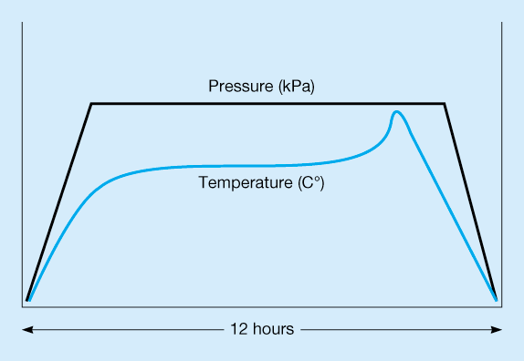
Figure 13.6 Temperature and Pressure Profile Example
Each furnace has a known yield rate with no noticeable variation according to the following:
| FURNACE | A | B | C | D | E | F | G | H | I | J | K | L |
|---|---|---|---|---|---|---|---|---|---|---|---|---|
| Yield | 0.95 | 0.975 | 0.975 | 0.975 | 0.975 | 0.975 | 0.975 | 0.995 | 0.995 | 0.995 | 0.995 | 0.999 |
That is to say, 1 in 20 batches fails at Furnace A and must be scrapped, whereas only 1 in 1,000 batches fails at Furnace L. As one might expect, upstream batch failures are very disruptive to the downstream operations. Scrapping batches causes downstream furnaces to sit idle under the current “zero in queue” work in process (WIP) inventory policy as they wait for good batches to arrive from upstream operations.
Design, build, and perform a 1,000-day simulation model study of the system described above in Excel, incorporating the random number generator function, RAND(). Start your simulation with a fully loaded furnace deck.
Discussion Questions
Determine and comment on the overall yield (the number of batches that make it all the way through Furnace L divided by the number that started at Furnace A) of disc brakes at FB Badpoore.
Determine the utilization of Furnace L.
Suggest improvements to the system.