19. Using Functions

A function is like a shortcut for using a long or complex formula. If you’ve ever summed cells by adding them individually (as in =A1+A2+A3+A4+A5), you could have instead used a SUM function like this: =SUM(A1:A5). Excel offers more than 400 functions. These include logical functions, lookup functions, statistical functions, financial functions, and more.

This chapter shows you how to look up functions available in Excel and reviews some functions helpful for everyday use.

Normally, the syntax of a function is like this:

FunctionName(Argument1, Argument2, ...)

But there are some functions that have no arguments or the argument is optional. There are a few rules to keep in mind when using functions:

• Arguments must be entered in the order required by the function.

• Arguments must be separated by commas.

• Arguments can be cell references, numbers, logicals, or text.

• Some arguments are optional. Optional arguments are placed after the required ones.

• If you skip an optional argument to use one after it, you still have to place a comma for the one you skipped.

• Some functions, such as NOW(), do not require arguments, but the parentheses must still be included in the formula.

The Formulas tab has a Function Library group with drop-downs grouped by function type. Selecting any function listed in a drop-down opens it up in the Formula Wizard.

If you aren’t sure which function you need, or if you need more help in using a function, there are several ways to open the Insert Function dialog box, which helps you find the required function:

• On the Home tab or Formulas tab, click the arrow below the AutoSum button and select More Functions from the menu.

• On the Formulas tab, click another button in the Function Library group and select Insert Function from the menu.

• On the Formulas tab, click the Insert Function button in the Function Library group.

• Click the fx button by the formula bar.

When you click Insert Function, the dialog box shown in Figure 19.1 opens. You can enter a search term in the Search for a Function field or select a category from the drop-down. Results appear in the list box. When you select a function from the list box, the arguments and a brief description of the function appear. When you find the function you want to use, highlight it and click OK. The function appears in the active cell and the Function Arguments dialog box opens, ready to help you fill in the rest of the arguments.

FIGURE 19.1 The Insert Function dialog box helps search through Excel’s more than 400 available functions.

FIGURE 19.2 The Function Arguments dialog box helps with the arguments of the selected function.

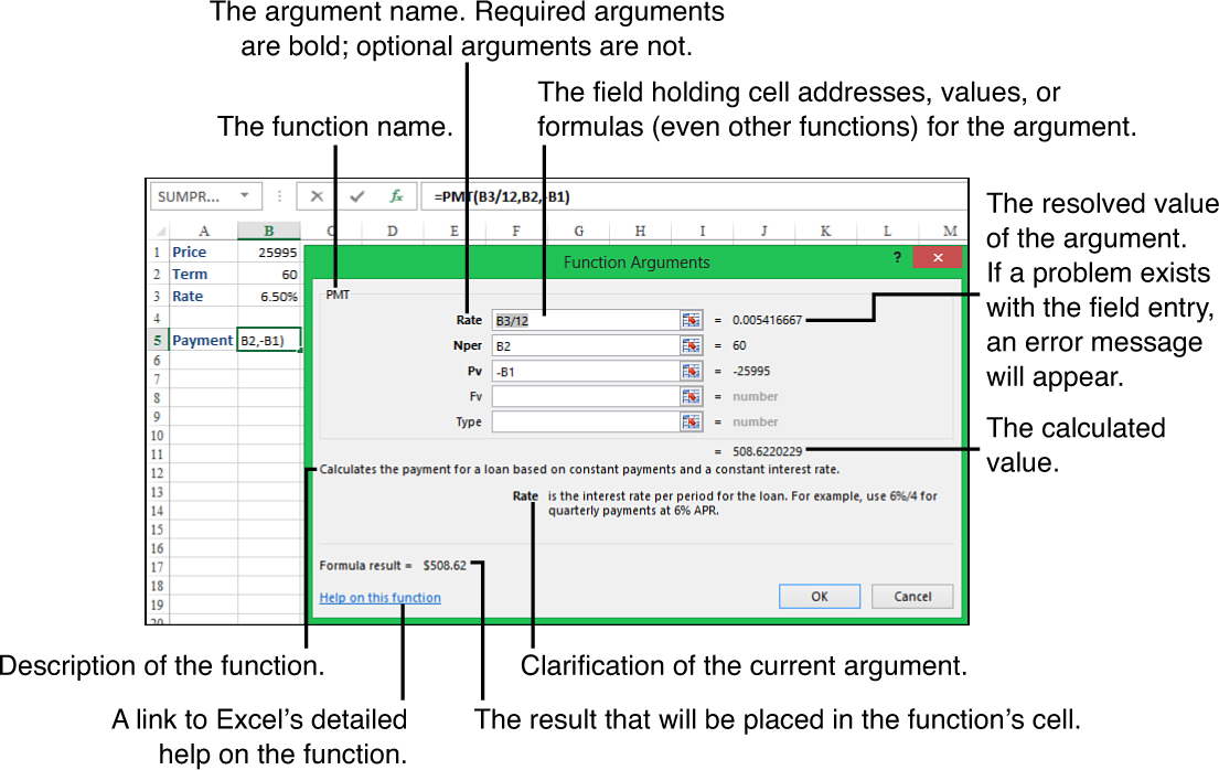
A field exists for each argument. If the function has a variable number of arguments, like the SUM function, a new field is automatically added when needed. The following list identifies the parts of the Function Arguments dialog box shown in Figure 19.2:

Figure 19.2 shows the PMT function being using to calculate the monthly payment for a loan. The loan amount is in cell B1, the number of months in cell B2, the APR in cell B3. The function is in cell B5. To insert the function and select its arguments, follow these steps:

1. Select the cell that holds the formula (cell B5).

2. On the Formulas tab, click the Insert Function button. In the Search field, type PMT and click Go.

3. PMT displays in the list of functions. Highlight it and click OK. The Function Arguments dialog box opens. If the dialog box is covering the values on the sheet (B1:B3), then click the title of the dialog box and drag it out of the way.

4. The first argument is Rate, the interest rate. When you click in the field and look at the description, notice it says this is the interest rate per period. Because your value is the annual rate, you need to divide it by 12. But first, you need to select it on the sheet. Click cell B3 and the cell address appears in the Rate field with the cursor blinking at the end of it. Enter /12 to get the monthly rate.

5. The second argument is the Nper, number of payments for the loan. First click the field in the dialog box and then select cell B2 on the sheet.

6. Click in the Pv field (present value of the loan) in the dialog box. Before selecting the cell on the sheet, enter a – (a minus sign) so that when you do click the cell on the sheet, you are making the value negative. You do this because of the way the function works. If you didn’t make this value negative, the payment itself would be negative.

7. Fv (future value after the last payment is made) and Type (–1 when the payment is made at the beginning of the period, 0 when it’s made at the end of the period) are both optional arguments and can be left blank.

8. If you do not see any error messages in the calculated value in the dialog box, click OK to have the cell accept the formula.

After you select the function, an in-cell tip appears, as shown in Figure 19.3. The current argument is bold. Optional arguments appear in square brackets. If you want to use the Function Arguments dialog box, press Ctrl+A after typing the function name in the cell. For more help with the function, click the function name in the tip, and Excel’s detailed Help file for the function appears.

FIGURE 19.3 If you’re already familiar with the function, you can use the in-cell help to guide you in filling out the arguments.

To type a function, such as SUM, directly into a cell, follow these steps:

1. Select the cell where you want to place the formula.

2. Type an equal sign.

3. Begin typing the name of the function. When the drop-down list appears, you can continue typing or scroll the list to highlight the function and press Tab.

4. Enter the first argument. The argument can be a cell address (you can type it or select it on the sheet), a value, or a formula.

5. If there is another argument, type a comma and then enter the next argument. Repeat this step for each argument. As you enter each argument, notice that the argument becomes bold in the in-cell tip, showing you your position in the function.

6. When you’re finished entering all the arguments, type the closing parenthesis and press Enter or Tab for the cell to accept the formula.

• Select a cell adjacent to the range and click the AutoSum button.

• Highlight the range including the adjacent cell where you want the formula placed, and then click the AutoSum button.

• If you need to sum multiple ranges, select the entire table, including the adjacent row or column where you want results to appear, and then click the AutoSum button.

Unless you select the range you want to calculate, Excel guesses which cells you are trying to sum and highlights them. If the selection is correct, press Enter to accept the solution. If the selection is incorrect, make the required changes and then press Enter to accept the solution.

You should keep an eye out for a couple of things when using the AutoSum function:

• Be careful of numeric headings (such as years) when letting Excel select the range for you. Excel cannot tell that the heading isn’t part of the calculation range, and you need to correct the selection before accepting the formula.

• Excel looks for a column to sum before summing a row. In Figure 19.4, the default selection by Excel is the numbers above the selected cell, instead of the adjacent row of numbers.

FIGURE 19.4 Excel defaults to calculating columns before rows. Instead of summing the West data, Excel selects the totals from East and Central instead.

1. Select B3:B6.

2. While holding down the Ctrl key, select B3:F3.

3. Click the AutoSum button.

4. Excel calculates and inserts the corresponding totals in the total cells.

FIGURE 19.5 Excel is smart enough to determine that you want to sum each individual row and column.

• Sum—Adds the values in the selected range (the default action)

• Average—Averages the values in the selected range

• Count Numbers—Returns the number of cells containing numbers

• Max—Returns the largest value in the selected range

• Min—Returns the smallest value in the selected range

These other options work on a range in the same way as the SUM function, but you have to select them from the drop-down, whereas with SUM, you can just click the button.

FIGURE 19.6 You can modify the status bar to show the results of calculations done to selected data.

To see the list of functions and be able to edit the values shown in the status bar, you must first select some data on a sheet. Next, right-click the status bar and the Customize Status Bar menu, shown in Figure 19.6, appears. You can toggle the check mark next to the functions you want to show or hide in the status bar. After you select the functions you want, whenever you select data, the resulting calculations appear in the status bar.

FIGURE 19.7 You can use the Quick Analysis tool to calculate a column, but not a row.