15. Excel 2013 Basics
In This Chapter
• Moving Around and Making Selections on a Sheet
• Using Templates to Quickly Create New Workbooks
• Working with Sheets and Tabs
• Working with Rows and Columns
Excel is a full-featured spreadsheet application that’s part of Microsoft Office 2013. With Excel, you can perform calculations, create charts, and analyze numerical data. An Excel file is called a workbook and each workbook can contain one or more sheets.
After exploring the Excel interface and its unique terminology, this chapter shows you how to create workbooks from scratch or from templates. It also shows you how to add, delete, and move sheets within a workbook or between workbooks.
Even a well-planned sheet layout might be missing something, such as a date column. Or you might change your mind in the middle of the design, deciding that you want a table elsewhere on a sheet. Instead of starting over, you learn how to insert rows or columns and move your tables to a new location on your sheet.
Exploring the Excel Window
When you open Excel 2013 for the first time, you see the Start screen, shown in Figure 15.1. This screen includes a list of Excel starter templates. (See “Using Templates to Quickly Create New Workbooks” later in this chapter for more details about templates.) For now, click the Blank Workbook item in the upper-left corner to open a blank spreadsheet, as shown in Figure 15.2.

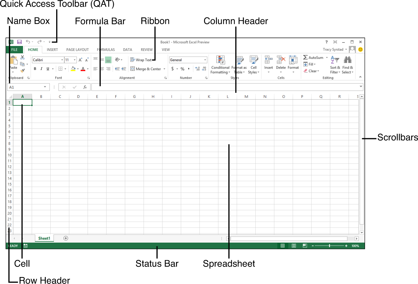
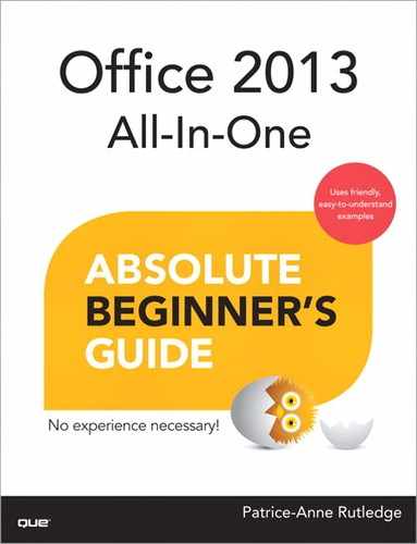
FIGURE 15.2 The Excel window is made up of many components that you use when working on a spreadsheet.
 Tip
Tip
To create a new workbook if you are already have another workbook open, click the File tab, select New, and then select Blank Workbook. Alternatively, you can press Ctrl+N on the keyboard. For more information about opening, closing, and saving files, see Chapter 2, “Working with Office Applications.”
The big grid taking up most of the Excel window is the spreadsheet, also known as a worksheet or, simply, a sheet. Each little box is a cell. Multiple cells selected together are commonly known as a range.
Right above the grid are letters known as column headers. Down the left side of the grid are numbers, also known as row headers. The intersection of a single column and a single row is a cell. Each cell has an address made up of the column letter and the row number. Figure 15.3 shows cell C8 selected. Note the C in the column header is highlighted as is the 8 in the row header.

FIGURE 15.3 The intersection of a column and a row is a cell. The cell gets its name from the column and row headers, in this case C8.
Above the headers and to the left is the Name box. This box shows you what you have selected on the sheet. This can be a cell address, a named range, a table, a chart, or some other object on the sheet. When you first open Excel, the Name box likely shows A1. If you select another cell on the sheet, the address changes to show that cell’s address, such as C8. Later in this chapter, you find out how you can use the Name box to quickly move to another area of the sheet.
To the right of the Name box is the formula bar, which is a slight misnomer. Although that is probably the most common use of this field, the formula bar actually reflects anything that’s been typed into a cell, not just formulas.
At the top of the Excel window, you find the Ribbon and the Quick Access Toolbar, which is covered in Chapter 1, “Getting Started with Microsoft Office 2013.”
Below and to the right of the grid are scrollbars, which you can use to move around the sheet. You can either click and drag a bar or use the arrows at either end of the scroll area.
The status bar is along the bottom of the Excel window. Not only does it show the status of Excel, such as Ready or Calculating, on the left side, but it also includes buttons for changing the page view or zoom. In the right corner of the status bar is the Zoom slider. You can use the slider or the – and + buttons to change the zoom of the active sheet.
To the left of the Zoom slider are three buttons for changing how you view the active sheet:
• Normal—This is the default view, showing just the sheet.
• Page Break Preview—Displays where columns and rows break to print onto other pages. Dashed lines signify automatic breaks that Excel places based on settings, such as margins. Solid lines are manually set breaks. See Chapter 22, “Preparing Workbooks for Distribution and Printing,” for more information on setting and moving page breaks.
• Page Layout—This view is similar to an editable Print Preview—you can see what your page looks like when it prints out, but you can still enter data and make other changes. Columns and rows move between pages as you adjust their widths or the margins of the page. You can also enter information directly into the header and footer of a page. See Chapter 22 for information on adding headers and footers.
Moving Around and Making Selections on a Sheet
You can move around on a sheet using the mouse or the keyboard, depending on which method is most comfortable for you. To select a cell using the mouse, click it. To select a cell using the keyboard, use the navigation arrows on the keyboard. You can also use the number keypad arrows if the NumLock feature is turned off.
Keyboard Shortcuts for Quicker Navigation
Using the navigation arrows on the keyboard can be a little slow, especially if you have a lot of cells between your currently selected cells and the one you want to select. Even using the mouse can take some time to navigate from the top of your data to the bottom. The following list details a few keyboard shortcuts to make navigation a little easier:
• Ctrl+Home jumps to cell A1, located at the upper-left corner of the sheet.
• Ctrl+End jumps to the last row and column in use.
• Ctrl+Left Arrow jumps to the first column with data to the left of the currently selected cell. If there is no data to the left then it selects a cell in the first column, A.
• Ctrl+Right Arrow jumps to the first column with data to the right of the currently selected cell. If there is no data to the right then it selects a cell in the last column, XFD.
• Ctrl+Down Arrow jumps to the first row with data below the currently selected cell. If there is no data below the selected cell then it selects a cell in the last row.
• Ctrl+Up Arrow jumps to the first row with data above the currently selected cell. If there is no data above the selected cell then it selects a cell in row 1.
Selecting a Range of Cells
You’ll often find yourself needing to select more than a single cell. For example, if you have text on a sheet you want to apply a new font to, instead of selecting one cell at a time and applying the font, you can select all the cells and then apply the font, as shown in Figure 15.4.

Tip
When selecting a range, it doesn’t matter if you start at the top or bottom or far left or far right of the range.
To select a range using the mouse, follow these steps:
1. Click in a cell in the corner of your selection.
2. Hold down the mouse button as you drag the mouse to cover the desired cells.
3. When you get to the last cell, let go of the mouse button. Excel selects a range similar to what is shown in Figure 15.4. As long as you don’t click elsewhere on the sheet, the range remains selected.
To select a range using the keyboard, follow these steps:
1. Click in a cell in the corner of your selection.
2. Press F8 on the keyboard.
3. Use the arrow keys to navigate to the end of the desired range.
4. Press F8 on the keyboard to stop the selection from extending. As long as you don’t select another cell on the sheet, the range remains selected.
 Note
Note
Pressing F8 on the keyboard activates the Extend Selection option in Excel. If you look at the left side of the status bar, you see Extend Selection. As long as the option is on, selecting different cells extends the selection.
Using Templates to Quickly Create New Workbooks
Templates are a great way for keeping data in a uniform design. You could simply design your workbook and reuse it as needed, but if you accidentally save data before you have renamed the file, your blank workbook is no longer clean. When using a template, there’s no risk of saving data in the template because you are working with a copy of the original workbook, not the workbook itself.
Using Microsoft’s Online Templates
Microsoft offers a variety of templates—such as budgets, invoices, and calendars—which can help you start a project. You can search for templates to fit your needs either from the Start screen or by clicking the File tab and selecting New to open the New screen, which displays a selection of templates. Alternatively, you can enter your own keywords in the Search field at the top of the New screen. A search returns matches, which you can filter from a list on the right.
Tip
When you place your cursor over a template preview, a pushpin appears in its lower-right corner, giving you the option to pin it so that it always appears in the list. If you found your template by searching for it, this is a way to make it easily accessible the next time you need it.
When you select a template, a preview window opens, as shown in Figure 15.5. The preview shows a larger example of the template, a brief explanation of its purpose, and how the template has been rated by other users. If you click Create, the template is downloaded (for first-time use) and opened.

FIGURE 15.5 Use the left and right arrows in the template preview window to scroll through other available templates before opening one.
Saving a Template
Note
You do not have to save templates to the configured templates location if you plan to double-click or right-click to open a copy of the file.
Before you can use your own template or one provided to you and not downloaded from the Office Store, you have to configure where to store your templates. This is a folder where you place all the templates you want to access through the New screen. To set up the location, click the File tab, select Options, and select the Save tab on the Excel Options dialog box. Next, enter the path in the Default Personal Templates Location field. After you have a location configured, the Personal link appears to the right of the Featured link on the New screen. Featured shows Microsoft’s online templates; Personal shows templates in the locally configured location.
 Caution
The location must exist before you enter it in the field. To make sure you get the path correct, navigate to it in File Explorer, copy the full path from the address bar, and then paste it in the Excel field.
Opening a Locally Saved Template to Enter Data
There are multiple ways to open a template to enter data, and you can use the method that is most convenient to you. To open a template to create a new workbook, use one of the following methods:
• Double-click the file from its saved location.
• From its saved location, right-click the file and select New.
• Click the File tab, select New, and select the template from the list of online templates.
• Click the File tab, select New, click the Personal link, and select from the list of templates saved locally. See the previous “Saving a Template” section for details on how to configure the location. The Personal option doesn’t appear unless you set up the location in the Excel Options dialog box.
Note
If you need to make changes to the design of a template, the previous methods for opening a copy of the template don’t work. Instead, to open the original template to make changes, right-click the file and select Open.
Working with Sheets and Tabs
A sheet, also known as a spreadsheet or worksheet, is where you enter your data in Excel. A workbook can have multiple sheets—the number is limited only by the power of the computer opening the workbook.
Each sheet has a tab, visible above the status bar, as shown in Figure 15.6. The sheet with data that you’re looking at is considered the active sheet. To select another sheet, click its tab.

FIGURE 15.6 The font of the sheet tab you are working on, Sheet1, is bold compared with the other sheet tabs.
Inserting a New Sheet
The quickest way to add a new sheet to a workbook is to click the circle with a plus sign that appears to the right of the rightmost sheet tab. This inserts a new sheet to the right of the active sheet.
To insert a new sheet to the left of a specific sheet, select the sheet (refer to the “Activating Another Sheet” section), click the Insert button on the Home tab, and select Insert Sheet from the menu.
A third method is to right-click the tab to the right of where you want the new sheet to appear. From the menu, select Insert, select Worksheet, and click OK. The new sheet appears to the left of the tab you right-clicked, as shown in Figure 15.7.

FIGURE 15.7 You can control where a new sheet is inserted by right-clicking a tab and selecting Insert.
Activating Another Sheet
To activate another sheet, click its tab along the bottom of the Excel window. You can also navigate sheet to sheet using the keyboard. Ctrl+Page Up selects the sheet to the left; Ctrl+Page Down selects the sheet to the right.
If you have more sheets than can fit in the tab area, three small dots appear on the left and right side of the area, to show there are more sheets available to view, as shown in Figure 15.7. Clicking the three dots quickly scrolls through multiple sheets. If instead, you need to scroll one sheet at a time, click the left and right arrows located to the left of the sheet tab area.
If you right-click the left and right arrows instead, a list of all sheets in the workbook appears. You can then select a sheet, click OK, and go straight to that sheet.
Selecting Multiple Sheets
You can select multiple sheets at one time. This doesn’t activate them all at once. It groups them together so that an action on one, such as changing the tab color, affects all of them.
To select multiple sheets, select the first one and then, while holding down the Ctrl key, select the tabs for the others. As you select each sheet tab, the sheet name becomes bold.
To ungroup the sheets, you can either select any sheet other than the active sheet or right-click any tab and select Ungroup Sheets.
Deleting a Sheet
If you no longer need a sheet, you can delete it, getting it out of your way and reducing the size of your workbook. To delete a sheet, right-click the sheet’s tab and select Delete. You can also delete a sheet by making it your active sheet, clicking the Delete button on the Home tab, and selecting Delete Sheet from the drop-down. If there is data on the sheet, a prompt appears to verify that you want to delete the sheet.
Caution
Deleting a sheet cannot be undone.
Moving or Copying Sheets Within the Same Workbook
You might want to reorganize sheets within the current workbook to group similar sheets together. Or you might need to copy a sheet to run tests on the data but don’t want to change the original. To move a sheet within a workbook, click the Format button on the Home tab and select Move or Copy Sheet from the menu. You can also access the Move or Copy dialog box by right-clicking a sheet tab and selecting Move or Copy.
In the Move or Copy dialog box, shown in Figure 15.8, make sure the To Book field is the current workbook. If you’re making a copy of the sheet, select the Create a Copy box. Then, in the Before Sheet dialog box, select the sheet you want the active sheet to be placed in front of (to the left of). You can also reorganize the sheets in a workbook by clicking, holding the mouse button down, and dragging the sheet’s tab to a new location. If you want to copy the sheet then hold down the Ctrl key as you move the sheet tab.

FIGURE 15.8 The Move or Copy dialog box enables you to copy or move sheets within a workbook or between two different workbooks.
Moving or Copying Sheets Between Workbooks
Many database programs export data to an Excel workbook or compatible file, but they might not let you choose an existing workbook to export to. If you have a report workbook designed in which you need the new data, you can copy or move the exported data from its workbook to your report workbook. To move a sheet to a new workbook, click the Format button on the Home tab and select Move or Copy Sheet from the menu. Alternatively, right-click a sheet tab and select Move or Copy.
To move or copy a sheet to another workbook, the second workbook must already be open. Make sure the sheet you want to move or copy is the active sheet. Then, using the Move or Copy dialog box, shown in Figure 15.8, select from the To Book field the workbook to move or copy the sheet to. If you’re making a copy of the sheet, select the Create a Copy box. In the Before Sheet dialog box, select the sheet you want the active sheet to be placed in front of (to the left of).
Caution
When you move or copy a sheet from one workbook to another, any formulas on that sheet linked to another sheet in the original workbook remain linked to the sheet in the original workbook unless you also include the linked sheet(s) in the move or copy procedure.
Renaming a Sheet
Excel’s sheet names, Sheet1, Sheet2, and so on, aren’t very descriptive. Also, when you copy a sheet in a workbook that already has a sheet by that name, Excel copies the sheet name, appending a number to the end of it. For example, if you copy Sheet1 within the same workbook, Excel renames it to Sheet1 (2). To give a sheet a more meaningful name, click the Format button on the Home tab and select Rename Sheet from the menu. Excel selects the current sheet name in the sheet’s tab, and you can type in the new name. You can also rename a sheet by right-clicking the sheet’s tab and selecting Rename.
Coloring a Sheet Tab
If you have several sheets you want to visually group together, you can color their tabs. For example, if you have some sheets that are for data input and others for reports, you could color your data input sheet tabs a light yellow and the report tabs a light blue.
To change the color of a tab, click the Format button on the Home tab, and select Tab Color from the menu. A selection of colors appears from which you can select the desired color. The tab color of the active sheet appears as a gradient but fills the entire tab for the other sheets. You can also change the tab color by right-clicking the tab and selecting Tab Color.
Working with Rows and Columns
It’s hard to create the perfect data table the first time around. There’s always something you’ve forgotten, such as the date column. Or maybe you did remember the date column but put it in the wrong place. Thankfully, you don’t have to start over. You can insert, delete, and move entire columns and rows with a few clicks of the mouse.
Selecting an Entire Row or Column
When you select an entire row or column on a sheet, you are selecting beyond what you can see on the sheet. You really do select the entire row or column and whatever you do to the part you can see affects the entire selection.
To select an entire row, place your cursor on the header until it turns into a single black arrow and then click the header for the row. For example, to select row 5, as shown in Figure 15.9, click the header 5. To select an entire column, click the header for the column.
If you need to select multiple, contiguous rows (or columns), click the first header and then, as you hold down the mouse button, drag the mouse down (or up) until you have selected all the rows you need. Let go of the mouse button and perform your desired action on the selection.
If you need to select multiple, noncontiguous rows (or columns), click the first header and then, as you hold down the Ctrl key, carefully click the headers of the other rows. When you’re done selecting, release the Ctrl key and perform your desired action on the selection.
Inserting an Entire Row and Column
You might want to insert a row if your data table is missing titles over the data. Or, you might need to insert a column if the data table is missing a column of information and you don’t want to enter the information at the end (right side) of the table. When you insert a row, Excel shifts the existing data down. When you insert a column, Excel shifts the existing data to the right.
Tip
If you select multiple rows or columns, Excel inserts that many rows or columns. For example, if you need to insert five new rows in your data, instead of highlighting one row, right-clicking and selecting Insert and then repeating this four more times, select five rows, right-click, and select Insert and—voila!—you have five blank rows. Note that the selection doesn’t have to be contiguous. For example, if you’ve selected several noncontiguous rows, Excel inserts one row beneath each selected row.
To insert a new row or column within an existing data set, select a cell in the row or column where you want the inserted row or column to go. For example, if you need to insert a new row 10, select a cell in row 10. On the Home tab, click the Insert button and select Insert Sheet Rows or Insert Sheet Columns. For a shortcut, you can right-click the row or column header and select Insert.
Deleting an Entire Row and Column
When you import data from another source, you might need to clean it up by deleting rows or columns of data you don’t need. When deleting a row, Excel shifts the data below the row up. For example, after deleting row 5, what was in row 6 now appears in row 5. If deleting a column, Excel shifts the data that was to the right of the deleted column to the left.
To delete a row or column, select a cell in the row or column to delete, click the Delete button on the Home tab, and select Delete Sheet Rows or Delete Sheet Columns. For a shortcut, you can right-click the row or column header and select Delete.
Tip
Your selection of rows or columns does not have to be contiguous. Excel deletes what you have selected.
Moving Entire Rows and Columns
You have to be careful when moving rows and columns. Depending on the method you use, you could end up overwriting other cells. To move rows or columns when you aren’t worried about overwriting existing data, follow these steps:
1. Select the row or column you want to move.
2. The selection is surrounded by a thick line. Place your cursor over the line until it turns into a four-headed arrow, as shown in Figure 15.10.

FIGURE 15.10 When the cursor changes to a four-headed arrow, you can click and drag the column to a new location.
3. Click on the line and hold the mouse button down.
4. Drag the selection to a new location and let go.
5. If there is any data in the new location, Excel asks if you want to overwrite it. If you say No, the move is canceled. The original row or column is still there, but it’s empty.
If you need to keep data in the new location intact, you could insert a row or column in the new location, copy the data to be moved, paste it in the inserted rows or columns and then go back to the original location, select it again, and delete it. Or, you could get it done more quickly by selecting and cutting the row or column, right-clicking the new location, and selecting Insert Cut Cells. Excel moves the data in the new location, inserting the cut data and also deleting the data in the old location.
To perform these actions using the Ribbon, after selecting and cutting the row or column, select a cell in the new location, click the Insert button on the Home tab, and select Insert Cut Cells from the menu.
Tip
With one small addition, you can use both of the previous methods to copy a row to a new location. If you’re using the drag method, hold down the Ctrl key as you drag the row to the other location. If you’re using the menu method, copy the row instead of cutting it and select Insert Copied Cells from the menu.
Working with Cells
Just like you can insert, move, and delete entire rows and columns, you can also insert, move, and delete cells. This section shows you how to quickly jump to a cell you can’t currently see on your sheet, select noncontiguous ranges, and insert, move, and delete cells.
Selecting a Cell Using the Name Box
Earlier in this chapter, you learned how each cell has an address made up of the column and row it resides in. You also explored navigation basics—either click a cell or use the keyboard to select a cell.
You can also jump to a cell by typing the cell address in the Name box, located above the sheet in the left corner. This is a great way of traveling quickly to a specific location on a large sheet.
To use this method, you must enter the cell address properly—that is, the column and then the row. For example, if you want to jump to cell AA33, you must type in AA33; you can’t type in 33AA. After typing the address, press Enter and the currently selected cell moves to cell AA33.
Selecting Noncontiguous Cells and Ranges
In the section “Selecting a Range of Cells” earlier in this chapter, you read about the basics of cell and range selection. In this section, you find out how to select multiple, noncontiguous ranges, as shown in Figure 15.11.

FIGURE 15.11 You can select noncontiguous cells by holding down the Ctrl key as you select each range.
You don’t always want to select cells right next to each other. For example, you might want to select only the cells with negative values and make them bold. You could select each cell one at a time and apply the bold format. Or, you could hold down the Ctrl key and select each cell. After you have selected all the cells, you let go of the Ctrl key and select your desired format (or other action).
Caution
When you select a cell using the Ctrl key method, you cannot deselect it. If you make a mistake in your cell selection, you have to start over.
Inserting Cells and Ranges
When you insert or delete rows and columns, Excel shifts all the data on the sheet. If you don’t want all the data shifted, select a specific range and then either right-click over the selection and choose Insert or click the Insert button on the Home tab and select Insert Cells from the menu. A prompt appears, asking you in which direction you want to shift your existing data, as shown in Figure 15.12. If you want to insert rows, choose Shift Cells Down. If you want to insert columns, choose Shift Cells Right.

FIGURE 15.12 You can control how much of a row or column is inserted by selecting a specific range beforehand.
Deleting Cells and Ranges
When you delete a range, you remove the cells from the sheet, shifting other data over to fill in the empty space. If you aren’t careful, you can ruin the careful layout of your sheet—for example, moving data from the credit column to the debit column. If what you really want is to delete the data in the cells, leaving the cells intact, Excel calls this clearing the contents. For specifics on clearing contents, see the section “Clearing the Contents of a Cell,” in Chapter 16, “Entering Sheet Data.”
To delete a range from a sheet, select the range and on the Home tab, click the Delete button and select Delete Cells from the menu. From the Delete dialog box that opens, choose whether you want to Shift Cells Left or Shift Cells Up. You can also open the dialog box by right-clicking the selected range and choosing Delete from the menu.
Moving Cells and Ranges
You have to be careful when moving a range—you could end up overwriting other cells. If you need to move rows or columns and aren’t worried about overwriting existing data, use the following method. If you don’t want to overwrite existing data in the new location, you need to use the Insert Cells method explained in the section “Inserting Cells and Ranges.” To move rows or columns when you aren’t worried about overwriting existing data, follow these steps:
1. Select the range you want to move.
2. The selection is surrounded by a thick line. Place your cursor over the line until it turns into a four-headed arrow, as shown in Figure 15.13.

3. Select the line and hold the mouse button down.
4. Drag the selection to a new location and let go.
5. If there is any data in the new location, Excel asks if you want to overwrite it. If you select No, Excel cancels the move. Select Yes to complete the move and clear the contents of the original range.