17. Formatting Sheets and Cells
In This Chapter
• Adjusting Row Heights and Column Widths
• Applying Conditional Formatting
• Using Cell Styles to Quickly Apply Formatting
• Using Themes to Ensure Uniformity in Design
Now that you have your data on a sheet, you need to format it so that it’s easy to decipher and readers can quickly make sense of it. From simple font formatting, wrapping text, and merging cells to placing icons in cells so it’s obvious how one number compares with another, Excel has the tools you need to make reports visually interesting.
 Note
Note
See Chapter 3, “Working with Text,” to learn about the cell formatting options in the Font group on the Home tab.
Adjusting Row Heights and Column Widths
If you can’t see all the data you enter in a cell or the data in a column doesn’t use up very much of the column width, you can adjust the column width as needed. Several methods are available for adjusting column widths on a sheet. Each method described here also works for adjusting row heights:
• Click and drag the border between the column headings—Place your cursor on the border between two column headings, as shown in Figure 17.1. When the cursor turns into two arrows, you can click and drag to the right to make the column to the left wider or drag to the left to make the column narrower. The advantage of this method is you have full control of the width of the column. The disadvantage is that it affects only one column.
• Double-click the border between the column headings—Excel automatically adjusts the left column to fit the widest value in that column. The advantage of this method is that the column is now wide enough to display all the contents. The disadvantage is if you have a cell with a very long entry, the new width might be impractical.
• Select multiple columns and drag the border for one column—The width of all the columns in the selection adjusts to the same width as the one you just adjusted.
• Select multiple columns and double-click the border for one column—Each column in the selection adjusts to accommodate its widest value.
• Apply one column’s width to other columns—If you have a column with a width you want other columns to have, you can copy that column and paste its width over the other columns by using the Column Widths option of the Paste Special dialog box.
• Use the controls on the ribbon—Select the column(s) to adjust, click the Format button on the Home tab, select Column Width, enter a width, and click OK.
• AutoFit a column to fit all the data below a title row—If you have a long title and need to fit the column to all the data below the title, double-clicking the border between column headings won’t work as this adjusts the column width based on the title. Instead, select the data in the column, without the title, and use the AutoFit Column Width option under Home, Cells, Format.
You can also use the Font Size drop-down list (found in the Font group on the Home tab) to adjust row height automatically. The default row height is based on the largest font size in the row. For example, if cell F2 has a font size of 26, even if there is no other text in the row, the row automatically adjusts to approximately 33. You can take advantage of this to set the height of a row, instead of manually setting the row height. The advantage is that when a user tries autofitting the row height, your setting won’t change.
Aligning Text in a Cell
The Alignment group on the Home tab consists of tools that affect how a value is situated in a cell or range. You can also access these controls from the Alignment tab of the Format Cells dialog box.
There are six alignment buttons in the Alignment group, representing the most popular settings for how a value is situated in a cell. Top Align, Middle Align, and Bottom Align describe the vertical placement of the value in the cell. Align Text Left, Center, and Align Text Right describe the horizontal placement of the value in the cell. More options are available in the Format Cells dialog box on the Alignment tab. The Mini toolbar has only one button for horizontal alignment, which centers the text of the selected cell.
Merging Two or More Cells
Merging cells takes two or more adjacent cells and combines them to make one cell. For example, if you are designing a form with many data entry cells and need space for a large comment area, resizing the column might not be practical as it also affects the size of the cells above it. Instead, select the range you want the comments to be entered in and merge the cells. Any text other than that found in the upper-left cell of the selection is deleted as the newly combined cell takes on the identity of this first cell.
On the Alignment tab in the Format Cells dialog box, there is a check box for Merge Cells. In the upper-right corner of the Mini toolbar is a toggle button (Merge/Unmerge) to merge and center the text of the selected range.
The Merge & Center drop-down in the Alignment group on the Home tab offers several options to merge cells in different ways:
• Merge & Center—This is the default action of the drop-down button. The selected cells will be merged and the text will be centered.
• Merge Across—If you have several rows where you want to merge the adjacent cells in the same row, you can select all the rows (and their adjacent columns to merge) and select Merge Across (see Figure 17.2).

FIGURE 17.2 Notice that although several rows are selected, using Merge Across kept the separate rows intact.
• Merge Cells—Equivalent to the check box in the Format Cells dialog box, the selected range will be merged, retaining the alignment of the upper-left cell in the selection.
• Unmerge Cells—Use this option to unmerge the selected cells.
Use caution when merging cells because it can lead to potential issues:
• Users will be unable to sort if there are merged cells within the data.
• Users will be unable to cut and paste unless the same cells are merged in the pasted location.
• Column and row AutoFit won’t work.
• Lookup type formulas return a match only for the first matching row or column.
 Tip
Tip
For an alternative to merging to get a title centered over a table, refer to the section “Centering Text Across a Selection.”
Centering Text Across a Selection
As noted in the preceding section, “Merging Two or More Cells,” merging cells can cause problems in Excel, limiting what you can do with a table. If you need to center text over several columns, instead of merging the cells, center the text across the multiple columns. To center a title across the top of a table without merging the cells, as shown in Figure 17.3, follow these steps:
1. Type your title in the leftmost cell to the table.
2. Select the title cell and extend the range to include all cells you want the title centered over.
3. Press Ctrl+1 or click the Format button on the Home tab and select Format Cells to open the Format Cells dialog box.
4. Select the Alignment tab.
5. From the Horizontal drop-down, select Center Across Selection.
6. Click OK.

Wrapping Text in a Cell to the Next Line
When you type a lot of text in a cell, it continues to extend to the right beyond the right border of the cell if there is nothing in the adjacent cell. You can widen the column to fit the text, but sometimes that might be impractical. If that’s the case, you can set the cell to wrap text, moving any text that extends past the edge of the column to a new line in the cell.
Normally, when you wrap a cell, the row height automatically adjusts to fit the text. If it doesn’t, make sure you don’t have the cell merged with another; Excel does not autofit merged cells. If there are merged cells, unmerge them and manually force an autofit (see the “Adjusting Row Heights and Column Widths” section). The row height begins to automatically adjust again.
To turn on text wrapping, select the cell and click the Wrap Text button on the Home tab or select Wrap Text on the Alignment tab of the Format Cells dialog box. There is no option on the Mini toolbar.
 Caution
If you manually adjust the row height any time before pasting, the height won’t adjust automatically. To reset the row so it adjusts automatically again, double-click the border between the desired row and the one beneath.
Indenting Cell Contents
By default, text entered in a cell is flush with the left side of the cell whereas numbers are flush to the right. To move a value away from the edge, you might be tempted to add spaces before or after the value. If you change your mind about this formatting at a later time, it can be quite tedious to remove the extraneous spaces.
Instead, use the Increase Indent and Decrease Indent buttons to move the value about two character lengths over. Increase Indent moves the value away from the edge it is aligned with. Decrease Indent moves the value back toward its edge.
Tip
If you use the Increase Indent and Decrease Indent buttons with a right-aligned number, the number becomes left-aligned and adjusts from the left margin. This does not occur with right-aligned text. To correct this, select the Alignment tab of the Format Cells dialog box, set the Horizontal alignment to Right, and then set the Indent value.
When adjusting the Indent from the Format Cells dialog box, the Alignment tab uses a single Indent field with a number to indicate the number of indentations. The Mini toolbar does not offer options for indenting.
Changing Text Orientation
Vertical text can be difficult to read, but sometimes limited space makes it a requirement. The Orientation button, which looks like ab written at a 45-degree angle, has multiple variations of Vertical Text, Angle Counterclockwise, Angle Clockwise, Vertical Text, Rotate Text Up, and Rotate Text Down. The Orientation section in Format Cells, Alignment offers more precise control (see Figure 17.4). There is no option on the Mini toolbar.

Formatting Numbers
The Number Format drop-down in the Number group of the Home tab has 11 formatting options available (General is the default). Figure 17.5 shows an example of each format.

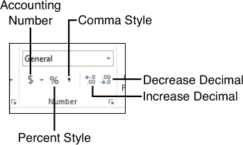
Below the Number Format drop-down is a drop-down button with a dollar sign ($) on it—the Accounting Number format. This button applies the accounting format to the selected range. From the drop-down, you can select different currency symbols.
Also beneath the drop-down are buttons for applying the Percent Style (%) and Comma Style (,) formats to a selection.
Use the Increase Decimal and Decrease Decimal buttons on the Home tab in the Number group (see Figure 17.6) to quickly increase and decrease the number of decimal places shown in number formats that use decimals. The Increase Decimal button has an arrow pointing left, whereas the Decrease Decimal button has an arrow pointing right.
Applying Number Formats with the Format Cells Dialog Box
The way you see number data in Excel is controlled by the format applied to the cell. For example, you might see the date as August 21, 2012, but what is actually in the cell is 41142. Or you might see 10.5%, but the actual value in the cell is 0.105. This is important because when doing calculations, Excel doesn’t care what you see. It deals only with the actual values.
There are only a few formatting options on the Home tab in the Number group. This section reviews the formatting options available on the Numbers tab of the Format Cells dialog box. (Click the dialog box launcher in the lower-right corner of the Number group to open.)
The Number tab includes a variety of number formatting options, described in this section. To apply a number format, select the range, select the desired format from the dialog box, and click OK.
General
General is the default format used by all cells on a sheet when you first open a workbook. Decimal places and the negative symbol are shown if needed. Thousand separators are not.
Number
By default, the Number format uses two decimal places but does not use the thousands separator. You can change the number of decimal places, turn on the thousands separator, and choose how to format negative numbers, as shown in Figure 17.7.

Currency
The default Currency format displays the system’s currency symbol, two decimal places, and a thousands separator. You can change the number of decimal places, change the currency symbol, and select a format for negative numbers.
Accounting
Accounting is similar to Currency but automatically lines up the currency symbols on the left side of the cell and decimal points to the right side of the cell. The default Accounting format displays the system’s currency symbol, two decimal places, and a thousands separator. You can change the number of decimal places and the currency symbol.
Date
There is no default Date format. Sometimes Excel reformats the date you enter; sometimes it keeps it the way you entered it. You can select a date format from the list in the Type box, which also contains date and time formats.
The date formats vary from short dates, such as 4/5, to long dates, such as Monday, April 5, 2010. When selecting a date format, look at the sample above the Type list. It helps you differentiate between the format 14-Mar, which is March 14, and the format Mar-01, which is March 2001, not March 1.
Time
There is no default Time format. You can select a time format from the list in the Type box, which also contains two date and time formats.
Excel sees times on a 24-hour clock. That is, if you enter 1:30, Excel assumes you mean 1:30 a.m. But if you enter 13:30, Excel knows you mean 1:30 p.m.
If you need to display times beyond 24 hours, such as if you’re working on a timesheet adding up hours worked, use the time format 37:30:55, as shown in Figure 17.8.

Percentage
The default Percentage format includes two decimal places. When you apply this format, Excel takes the value in the cell, multiplies it by 100, and adds a % at the end. When you use the cell in a calculation, the actual (decimal) value is used. For example, if you have a cell showing 90% and multiply it by 1,000, the result is (in General format) 900 (0.9*1,000).
If you include the % when you type the value in the cell, in the background Excel converts the value to its decimal equivalent, but the Percentage format is applied to the cell.
Fraction
The Fraction category rounds decimal numbers up to the nearest fraction. You can select to round the decimal to one, two, or three digits, or to round to the nearest half, quarter, eighth, sixteenth, tenth, or hundredth.
Scientific
The default Scientific category displays the value in scientific notation accurate to two decimal places. You can change the number of decimal places.
Text
There are no controls for the Text category. Setting this format to a cell forces Excel to treat the numbers in the cell as text, and you view exactly what is in the cell. If you set this format before typing in a number, the number becomes a number stored as text and might not work in some calculations.
Special
The Special category provides formats for numbers that do not fall in any of the preceding categories because the values are not actually numbers. That is, they aren’t used for any mathematical operations and instead are treated more like words.
The four special types are specific to U.S. formatting:
• ZIP Code—Ensures that East Coast cities do not lose the leading zeros in their ZIP Codes.
• ZIP Code + 4—Ensures that East Coast cities do not lose the leading zeros in their ZIP Codes and formats the +4 in ZIP codes.
• Phone Number—Formats a telephone number with parentheses around the area code and a dash after the exchange.
• Social Security Number—Uses hyphens to separate the digits into groups of three, two, and four numbers.
Custom Format
A custom format enables you to create a format specific to your situation and can contain up to four different formats, each separated by a semicolon.
You should keep several things in mind when creating a custom format:
• Use semicolons to separate the code sections.
• If there is only one format, it applies to all numbers.
• If there are two formats, the first section applies to positive and zero values. The second section applies to negative values.
• If there are three formats, the first section applies to positive values, the second section applies to negative values, and the third section applies to zero values.
• If all four sections are used, they apply to positive, negative, zero, and text values, respectively.
Figure 17.9 shows a custom number format using all four sections. The table in C9:D13 displays how the formats would be applied to different values. The M in in the first and second section adds an M to the numerical values. The @ in the fourth section is a placeholder for any text the user types into the cell. Note the value in cell D11 is red and a zero, not a blank, must be entered in cell C12 for “No Sales” to appear.

FIGURE 17.9 Use the four sections of a custom format to design formatting for positive, negative, zero, and text values.
Tip
If you see ### in a cell, try increasing the size of the column. Sometimes Excel doesn’t automatically adjust the column width for an entered number.
Creating Hyperlinks
Hyperlinks enable you to open web pages in your browser, create emails, and jump to a specific cell on a specific sheet in a specific workbook. For web and email addresses, Excel automatically recognizes what you’ve typed and applies the format accordingly, turning the cell into a clickable link.
If you want to link to a sheet, you have to go through the Insert Hyperlink dialog box, shown in Figure 17.10. You can open the dialog box by right-clicking on a cell and selecting Hyperlink or clicking the Hyperlink button on the Insert tab.

Being able to create a hyperlink to a sheet can be useful if you want to create a table of contents for a large workbook or a series of workbooks.
If you select just a sheet, Excel defaults to cell A1 on the sheet, but you can link to any specified cell. To create a hyperlink to a specific sheet, follow these steps:
1. Select the cell where you want the link.
2. On the Insert tab, click the Hyperlink button to open the Hyperlinks dialog box.
3. Browse to the workbook you want to link to. If you want to link to a cell in the current workbook, click the Place in This Document button.
4. If linking to an external workbook, click the Bookmark button to open the Select Place in Document dialog box. If linking to the active workbook, continue to step 5.
5. Select the sheet from the Cell Reference list. If you have a specific cell address you want the link to go to, enter it in the Type the Cell Reference field. Or, if you have a name assigned to the cell, select it from the Defined Names list. In that case, you don’t have to enter a cell reference.
7. If the cell selected in step 1 is blank, the Text to Display field at the top of the dialog box shows the destination for the hyperlink. You can type in new text if desired.
8. Click OK. The next time you click on the cell, you follow the link.
Applying Conditional Formatting
An unformatted sheet of just numbers isn’t going to grab your audience’s attention. But sometimes you don’t have time to create a colorful report—or do you? Conditional formatting enables you to quickly apply color and icons to data. The quick formatting options consist of the following:
• Data Bars—A data bar is a gradient or solid fill of color that starts at the left edge of the cell. The length of the bar represents the value in the cell compared with other values in the range the format is applied to. The smallest numbers have just a tiny amount of color and the largest numbers in the range fill the cell.
• Color Scales—A color scale is a color that fills the entire cell. Two or three different colors are used to relay the relative size of each cell to other cells in the range the format is applied to.
• Icon Sets—An icon set is a group of three to five images that provide a graphic representation of how the number in a cell compares with the other cells in the range the format is applied to.
The quickest way to apply one of the conditional formats is to select all the cells you want to apply it to, click the Conditional Formatting button on the Home tab and select one of the formatting options from the submenu that appears, as shown in Figure 17.11. As you move your cursor over the options, your range changes to reflect the connection. When you find the formatting you want, click it, and it is applied to your range.

FIGURE 17.11 Quickly apply formatting to your data by selecting one of the prebuilt options in the Conditional Formatting drop-down.
Tip
When you select a range of numbers, in the lower-right corner of the very last cell Excel’s Quick Analysis tool displays with several preset conditional formatting options to choose from.
Using Cell Styles to Quickly Apply Formatting
You’re probably used to using styles in Word but never realized that styles are also available in Excel. Select a range in Excel and click the Cell Styles button on the Home tab. Move your cursor over the predefined styles and watch your range update to reflect the styles.
You aren’t limited to these predefined styles. You can create and save your own style for use throughout the workbook it’s saved in. To quickly create a custom style in the active workbook, follow these steps:
1. Select a cell with all the formatting styles needed.
2. On the Home tab, click the Cell Styles button, and select New Cell Style.
3. If there is any type of formatting you do not want as part of the style, such as the alignment, unselect that style option.
4. Enter a name for the style in the Style Name field and click OK.
Using Themes to Ensure Uniformity in Design
Themes are collections of fonts, colors, and graphic effects that can be applied to a workbook. This can be useful if you have a series of company reports that need to have the same color and fonts. Only one theme can affect a workbook at a time.
Excel includes several built-in themes, which you can access from the Themes drop-down under Page Layout, Themes. You can also create and share themes you design.
A theme has the following components, which you can apply individually, instead of applying an entire Theme package:
• Fonts—A theme includes a font for headings and a font for body text.
• Colors—There are 12 colors in a theme: 4 for text, 6 for accents, and 2 for hyperlinks.
• Graphic effects—Graphic effects include lines, fills, bevels, shadows, and so on.
Applying a New Theme
The Themes group on the Page Layout tab has four buttons:
• Themes—Enables you to switch themes or save a new one
• Colors—Enables you to select a new color palette from the available built-in themes
• Fonts—Enables you to select a new font palette from the available built-in themes
• Effects—Enables you to select a new effect from the available built-in themes
Before applying a theme, arrange the sheet so you can see any themed elements such as charts or SmartArt. Then click the Themes button on the Page Layout tab and watch the elements update as you move your cursor over the various themes in the Themes drop-down. When you find the one you like, click it, and it will be applied to the workbook.
If you just want to change a theme component, make a selection from the component’s drop-down in the same way you would a theme.
Creating a New Theme
To create a new theme, you need to specify the colors and fonts and select an effect from the respective component’s drop-down. Then, under the Themes drop-down, choose Save Current Theme to save the theme.
To create a new theme, follow these steps:
1. On the Page Layout tab, click the Colors button, and select Customize Colors.
2. To change an item’s color, such as Accent 5 in Figure 17.12, choose its drop-down to open the color chooser.

3. When you find the desired color, click it to apply it to your theme.
4. Repeat steps 2 and 3 for each color you want to change.
5. In the Name field at the bottom, type a name for your color theme.
6. Click Save.
7. On the Page Layout tab, click the Fonts button, and select Customize Fonts.
8. To change the Heading font, choose its drop-down to open the font list.
9. When you find the desired font, click it to apply it to your theme. The Sample box on the right updates to reflect your selection.
10. Repeat steps 8 and 9 for the Body font.
11. In the Name field at the bottom, type a name for your font theme.
12. Click Save.
13. On the Page Layout tab, click the Effects button.
14. Select an effect from the gallery of built-in effects.
15. On the Page Layout tab, click the Themes button, and select Save Current Theme.
16. Browse to where you want to save the theme, type a name for it, and click Save.
Sharing a Theme
To share a theme with other people, you must send them the *.thmx file you saved when you created the theme.
When they receive the file, they should save it to either their equivalent theme folder or some other location by clicking the Themes button on the Page Layout tab and selecting Browse for Themes.