20.3 Sorting Algorithms
Sorting data (i.e., placing the data into some particular order, such as ascending or descending) is one of the most important computing applications. A bank sorts all of its checks by account number so that it can prepare individual bank statements at the end of each month. Telephone companies sort their lists of accounts by last name and, further, by first name to make it easy to find phone numbers. Virtually every organization must sort some data, and often, massive amounts of it. Sorting data is an intriguing, computer-intensive problem that has attracted intense research efforts.
An important point to understand about sorting is that the end result—the sorted array—will be the same no matter which algorithm you use to sort the array. Your algorithm choice affects only the algorithm’s runtime and memory use. The next two sections introduce the selection sort and insertion sort—simple algorithms to implement, but inefficient. In each case, we examine the efficiency of the algorithms using Big O notation. We then present the merge sort algorithm, which is much faster but is more difficult to implement.
20.3.1 Insertion Sort
Figure 20.4 uses insertion sort—a simple, but inefficient, sorting algorithm—to sort a 10-element array’s values into ascending order. Function template insertionSort (lines 9–25) implements the algorithm.


Fig. 20.4 Sorting an array into ascending order with insertion sort.
Alternate View
 1   // Fig. 20.4: InsertionSort.cpp
 2   // Sorting an array into ascending order with insertion sort.
 3   #include <array>
 4   #include <iomanip>
 5   #include <iostream>
 6   using namespace std;
 7
 8   // sort an array into ascending order
 9   template <typename T, size_t size>
10   void insertionSort(array<T, size>& items) {
11      // loop over the elements of the array
12      for (size_t next{1}; next < items.size(); ++next) {
13         T insert{items[next]}; // save value of next item to insert
14         size_t moveIndex{next}; // initialize location to place element
15
16         // search for the location in which to put the current element
17         while ((moveIndex > 0) && (items[moveIndex - 1] > insert)) {
18            // shift element one slot to the right
19            items[moveIndex] = items[moveIndex - 1];
20            --moveIndex;
21         }
22
23         items[moveIndex] = insert; // place insert item back into array
24      }
25   }
26
27   int main() {
28      const size_t arraySize{10}; // size of array
29      array<int, arraySize> data{34, 56, 4, 10, 77, 51, 93, 30, 5, 52};
30
31      cout << "Unsorted array:
";
32
33      // output original array
34      for (size_t i{0}; i < arraySize; ++i) {
35         cout << setw(4) << data[i];
36      }
37
38      insertionSort(data); // sort the array
39
40      cout << "
Sorted array:
";
41
42      // output sorted array
43      for (size_t i{0}; i < arraySize; ++i) {
44         cout << setw(4) << data[i];
45      }
46
47      cout << endl;
48   }
Unsorted array:
  34  56   4  10  77  51  93  30   5  52
Sorted array:
   4   5  10  30  34  51  52  56  77  93
Insertion Sort Algorithm
The algorithm’s first iteration takes the array’s second element and, if it’s less than the first element, swaps it with the first element (i.e., the algorithm inserts the second element in front of the first element). The second iteration looks at the third element and inserts it into the correct position with respect to the first two elements, so all three elements are in order. At the ith iteration of this algorithm, the first i elements in the original array will be sorted.
First Iteration
Line 29 declares and initializes the array named data with the following values:
34 56 4 10 77 51 93 30 5 52
Line 38 passes the array to the insertionSort function, which receives the array in parameter items. The function first looks at items[0] and items[1], whose values are 34 and 56, respectively. These two elements are already in order, so the algorithm continues—if they were out of order, the algorithm would swap them.
Second Iteration
In the second iteration, the algorithm looks at the value of items[2] (that is, 4). This value is less than 56, so the algorithm stores 4 in a temporary variable and moves 56 one element to the right. The algorithm then determines that 4 is less than 34, so it moves 34 one element to the right. At this point, the algorithm has reached the beginning of the array, so it places 4 in items[0]. The array now is
4 34 56 10 77 51 93 30 5 52
Third Iteration and Beyond
In the third iteration, the algorithm places the value of items[3] (that is, 10) in the correct location with respect to the first four array elements. The algorithm compares 10 to 56 and moves 56 one element to the right because it’s larger than 10. Next, the algorithm compares 10 to 34, moving 34 right one element. When the algorithm compares 10 to 4, it observes that 10 is larger than 4 and places 10 in items[1]. The array now is
4 10 34 56 77 51 93 30 5 52
Using this algorithm, after the ith iteration, the first i + 1 array elements are sorted. They may not be in their final locations, however, because the algorithm might encounter smaller values later in the array.
Function Template insertionSort
Function template insertionSort performs the sorting in lines 12–24, which iterates over the array’s elements. In each iteration, line 13 temporarily stores in variable insert the value of the element that will be inserted into the array’s sorted portion. Line 14 declares and initializes the variable moveIndex, which keeps track of where to insert the element. Lines 17–21 loop to locate the correct position where the element should be inserted. The loop terminates either when the program reaches the array’s first element or when it reaches an element that’s less than the value to insert. Line 19 moves an element to the right, and line 20 decrements the position at which to insert the next element. After the while loop ends, line 23 inserts the element into place. When the for statement in lines 12–24 terminates, the array’s elements are sorted.
Big O: Efficiency of Insertion Sort
Insertion sort is simple, but inefficient, sorting algorithm. This becomes apparent when sorting large arrays. Insertion sort iterates times, inserting an element into the appropriate position in the elements sorted so far. For each iteration, determining where to insert the element can require comparing the element to each of the preceding elements—n – 1 comparisons in the worst case. Each individual iteration statement runs in O(n) time. To determine Big O notation, nested statements mean that you must multiply the number of comparisons. For each iteration of an outer loop, there will be a certain number of iterations of the inner loop. In this algorithm, for each O(n) iteration of the outer loop, there will be O(n) iterations of the inner loop, resulting in a Big O of O(n * n) or .
20.3.2 Selection Sort
Figure 20.5 uses the selection sort algorithm—another easy-to-implement, but inefficient, sorting algorithm—to sort a 10-element array’s values into ascending order. Function template selectionSort (lines 9–27) implements the algorithm.


Fig. 20.5 Sorting an array into ascending order with selection sort.
Alternate View
 1   // Fig. 20.5: fig20_05.cpp
 2   // Sorting an array into ascending order with selection sort.
 3   #include <array>
 4   #include <iomanip>
 5   #include <iostream>
 6   using namespace std;
 7
 8   // sort an array into ascending order
 9   template <typename T, size_t size>
10   void selectionSort(array<T, size>& items) {
11      // loop over size - 1 elements
12      for (size_t i{0}; i < items.size() - 1; ++i) {
13         size_t indexOfSmallest{i}; // will hold index of smallest element
14
15         // loop to find index of smallest element
16         for (size_t index{i + 1}; index < items.size(); ++index) {
17            if (items[index] < items[indexOfSmallest]) {
18               indexOfSmallest = index;
19            }
20         }
21
22         // swap the elements at positions i and indexOfSmallest
23         T hold{items[i]};
24         items[i] = items[indexOfSmallest];
25         items[indexOfSmallest] = hold;
26      }
27   }
28
29   int main() {
30      const size_t arraySize{10};
31      array<int, arraySize> data{34, 56, 4, 10, 77, 51, 93, 30, 5, 52};
32
33      cout << "Unsorted array:
";
34
35      // output original array
36      for (size_t i{0}; i < arraySize; ++i) {
37         cout << setw(4) << data[i];
38      }
39
40      selectionSort(data); // sort the array
41
42      cout << "
Sorted array:
";
43
44      // output sorted array
45      for (size_t i{0}; i < arraySize; ++i) {
46         cout << setw(4) << data[i];
47      }
48
49      cout << endl;
50   }
Unsorted array:
  34  56   4  10  77  51  93  30   5  52
Sorted array:
   4   5  10  30  34  51  52  56  77  93
Selection Sort Algorithm
The algorithm’s first iteration selects the smallest element value and swaps it with the first element’s value. The second iteration selects the second-smallest element value (which is the smallest of the remaining elements) and swaps it with the second element’s value. The algorithm continues until the last iteration selects the second-largest element and swaps it with the second-to-last element’s value, leaving the largest value in the last element. After the ith iteration, the smallest i values will be sorted into increasing order in the first i array elements.
First Iteration
Line 31 declares and initializes the array named data with the following values:
34 56 4 10 77 51 93 30 5 52
The selection sort first determines the smallest value (4) in the array, which is in element 2. The algorithm swaps 4 with the value in element 0 (34), resulting in
4 56 34 10 77 51 93 30 5 52
Second Iteration
The algorithm then determines the smallest value of the remaining elements (all elements except 4), which is 5, contained in element 8. The program swaps the 5 with the 56 in element 1, resulting in
4 5 34 10 77 51 93 30 56 52
Third Iteration
On the third iteration, the program determines the next smallest value, 10, and swaps it with the value in element 2 (34).
4 5 10 34 77 51 93 30 56 52
The process continues until the array is fully sorted.
4 5 10 30 34 51 52 56 77 93
After the first iteration, the smallest element is in the first position; after the second iteration, the two smallest elements are in order in the first two positions and so on.
Function Template selectionSort
Function template selectionSort performs the sorting in lines 12–26. The loop iterates size - 1 times. Line 13 declares and initializes the variable indexOfSmallest, which stores the index of the smallest element in the unsorted portion of the array. Lines 16–20 iterate over the remaining array elements. For each element, line 17 compares the current element’s value to the value at indexOfSmallest. If the current element is smaller, line 18 assigns the current element’s index to indexOfSmallest. When this loop finishes, indexOfSmallest contains the index of the smallest element remaining in the array. Lines 23–25 then swap the elements at positions i and indexOfSmallest, using the temporary variable hold to store items[i]’s value while that element is assigned items[indexOfSmallest].
Efficiency of Selection Sort
The selection sort algorithm iterates times, each time swapping the smallest remaining element into its sorted position. Locating the smallest remaining element requires comparisons during the first iteration, during the second iteration, then , 2, 1. This results in a total of or comparisons. In Big O notation, smaller terms drop out and constants are ignored, leaving a Big O of . Can we develop sorting algorithms that perform better than ?
20.3.3 Merge Sort (A Recursive Implementation)
Merge sort is an efficient sorting algorithm but is conceptually more complex than insertion sort and selection sort. The merge sort algorithm sorts an array by splitting it into two equal-sized sub-arrays, sorting each sub-array then merging them into one larger array. With an odd number of elements, the algorithm creates the two sub-arrays such that one has one more element than the other.
Merge sort performs the merge by looking at each sub-array’s first element, which is also the smallest element in that sub-array. Merge sort takes the smallest of these and places it in the first element of merged sorted array. If there are still elements in the sub-array, merge sort looks at the second element in that sub-array (which is now the smallest element remaining) and compares it to the first element in the other sub-array. Merge sort continues this process until the merged array is filled. Once a sub-array has no more elements, the merge copies the other array’s remaining elements into the merged array.
Sample Merge
Suppose the algorithm has already merged smaller arrays to create sorted arrays A:
4 10 34 56 77
and B:
5 30 51 52 93
Merge sort merges these arrays into a sorted array. The smallest value in A is 4 (located in the zeroth element of A). The smallest value in B is 5 (located in the zeroth element of B). In order to determine the smallest element in the larger array, the algorithm compares 4 and 5. The value from A is smaller, so 4 becomes the value of the first element in the merged array. The algorithm continues by comparing 10 (the value of the second element in A) to 5 (the value of the first element in B). The value from B is smaller, so 5 becomes the value of the second element in the larger array. The algorithm continues by comparing 10 to 30, with 10 becoming the value of the third element in the array, and so on.
Recursive Implementation
Our merge sort implementation is recursive. The base case is an array with one element. Such an array is, of course, sorted, so merge sort immediately returns when it’s called with a one-element array. The recursion step splits an array of two or more elements into two equal-sized sub-arrays, recursively sorts each sub-array, then merges them into one larger, sorted array. [Again, if there is an odd number of elements, one sub-array is one element larger than the other.]
Demonstrating Merge Sort
Figure 20.6 implements and demonstrates the merge sort algorithm. Throughout the program’s execution, we use function template displayElements (lines 10–22) to display the portions of the array that are currently being split and merged. Function templates mergeSort (lines 25–48) and merge (lines 51–98) implement the merge sort algorithm. Function main (lines 100–125) creates an array, populates it with random integers, executes the algorithm (line 120) and displays the sorted array. The output from this program displays the splits and merges performed by merge sort, showing the progress of the sort at each step of the algorithm.


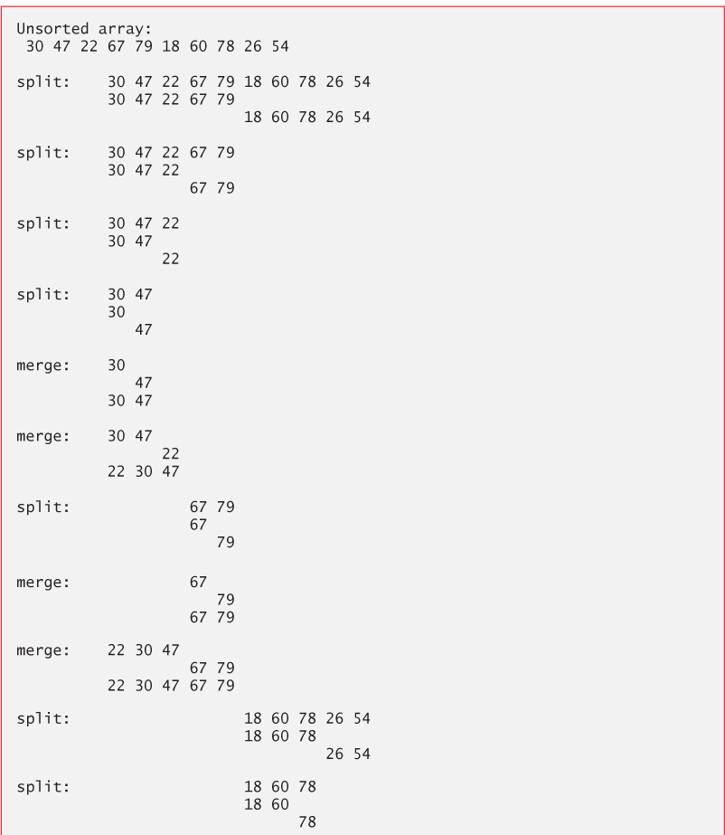

Fig. 20.6 Sorting an array into ascending order with merge sort.
Alternate View
  1   // Fig 20.6: Fig20_06.cpp
  2   // Sorting an array into ascending order with merge sort.
  3   #include <array>
  4   #include <ctime>
  5   #include <iostream>
  6   #include <random>
  7   using namespace std;
  8
  9   // display array elements from index low through index high
 10   template <typename T, size_t size>
 11   void displayElements(const array<T, size>& items,
 12      size_t low, size_t high) {
 13      for (size_t i{0}; i < items.size() && i < low; ++i) {
 14         cout << " "; // display spaces for alignment
 15      }
 16
 17      for (size_t i{low}; i < items.size() && i <= high; ++i) {
 18         cout << items[i] << " "; // display element
 19      }
 20
 21      cout << endl;
 22   }
 23
 24   // split array, sort subarrays and merge subarrays into sorted array
 25   template <typename T, size_t size>
 26   void mergeSort(array<T, size>& items, size_t low, size_t high) {
 27      // test base case; size of array equals 1
 28      if ((high - low) >= 1) { // if not base case
 29         size_t middle1{(low + high) / 2}; // calculate middle of array
 30         size_t middle2{middle1 + 1}; // calculate next element over
 31
 32         // output split step
 33         cout << "split: ";
 34         displayElements(items, low, high);
 35         cout << " ";
 36         displayElements(items, low, middle1);
 37         cout << " ";
 38         displayElements(items, middle2, high);
 39         cout << endl;
 40
 41         // split array in half; sort each half (recursive calls)
 42         mergeSort(items, low, middle1); // first half of array
 43         mergeSort(items, middle2, high); // second half of array
 44
 45         // merge two sorted arrays after split calls return
 46         merge(items, low, middle1, middle2, high);
 47      }
 48   }
 49
 50   // merge two sorted subarrays into one sorted subarray
 51   template <typename T, size_t size>
 52   void merge(array<T, size>& items,
 53      size_t left, size_t middle1, size_t middle2, size_t right) {
 54      size_t leftIndex{left}; // index into left subarray
 55      size_t rightIndex{middle2}; // index into right subarray
 56      size_t combinedIndex{left}; // index into temporary working array
 57      array<T, size> combined; // working array
 58
 59      // output two subarrays before merging
 60      cout << "merge: ";
 61      displayElements(items, left, middle1);
 62      cout << " ";
 63      displayElements(items, middle2, right);
 64      cout << endl;
 65
 66      // merge arrays until reaching end of either
 67      while (leftIndex <= middle1 && rightIndex <= right) {
 68         // place smaller of two current elements into result
 69         // and move to next space in array
 70         if (items[leftIndex] <= items[rightIndex]) {
 71            combined[combinedIndex++] = items[leftIndex++];
 72         }
 73         else {
 74            combined[combinedIndex++] = items[rightIndex++];
 75         }
 76      }
 77
 78      if (leftIndex == middle2) { // if at end of left array
 79         while (rightIndex <= right) { // copy in rest of right array
 80            combined[combinedIndex++] = items[rightIndex++];
 81         }
 82      }
 83      else { // at end of right array
 84         while (leftIndex <= middle1) { // copy in rest of left array
 85            combined[combinedIndex++] = items[leftIndex++];
 86         }
 87      }
 88
 89      // copy values back into original array
 90      for (size_t i = left; i <= right; ++i) {
 91         items[i] = combined[i];
 92      }
 93
 94      // output merged array
 95      cout << " ";
 96      displayElements(items, left, right);
 97      cout << endl;
 98   }
 99
100   int main() {
101      // use the default random-number generation engine to produce
102      // uniformly distributed pseudorandom int values from 10 to 99
103      default_random_engine engine{
104         static_cast<unsigned int>(time(nullptr))};
105      uniform_int_distribution<unsigned int> randomInt{10, 99};
106
107      const size_t arraySize{10}; // size of array
108      array<int, arraySize> data; // create array
109
110      // fill data with random values
111      for (int &item : data) {
112         item = randomInt(engine);
113      }
114
115      // display data's values before mergeSort
116      cout << "Unsorted array:" << endl;
117      displayElements(data, 0, data.size() - 1);
118      cout << endl;
119
120      mergeSort(data, 0, data.size() - 1); // sort the array data
121
122      // display data's values after mergeSort
123      cout << "Sorted array:" << endl;
124      displayElements(data, 0, data.size() - 1);
125   }
Unsorted array:
 30 47 22 67 79 18 60 78 26 54

split:    30 47 22 67 79 18 60 78 26 54
          30 47 22 67 79
                         18 60 78 26 54

split:    30 47 22 67 79
          30 47 22
                   67 79

split:    30 47 22
          30 47
                22

split:   30 47
         30
            47

merge:   30
            47
         30 47

merge:   30 47
               22
         22 30 47

split:            67 79
                  67
                     79


merge:            67
                     79
                  67 79

merge:   22 30 47
                  67 79
         22 30 47 67 79

split:                  18 60 78 26 54
                        18 60 78
                                 26 54

split:                  18 60 78
                        18 60
                              78

split:                  18 60
                        18
                           60

merge:                  18
                           60
                        18 60

merge:                  18 60
                              78
                        18 60 78

split:                           26 54
                                 26
                                    54

merge:                           26
                                    54
                                 26 54

merge:                  18 60 78
                                 26 54
                        18 26 54 60 78

merge:   22 30 47 67 79
                        18 26 54 60 78
         18 22 26 30 47 54 60 67 78 79

Sorted array:
 18 22 26 30 47 54 60 67 78 79
Function mergeSort
Recursive function mergeSort (lines 25–48) receives as parameters the array to sort and the low and high indices of the range of elements to sort. Line 28 tests the base case. If the high index minus the low index is 0 (i.e., a one-element sub-array), the function simply returns. If the difference between the indices is greater than or equal to 1, the function splits the array in two—lines 29–30 determine the split point. Next, line 42 recursively calls function mergeSort on the array’s first half, and line 43 recursively calls function mergeSort on the array’s second half. When these two function calls return, each half is sorted. Line 46 calls function merge (lines 51–98) on the two halves to combine the two sorted arrays into one larger sorted array.
Function merge
Lines 67–76 in function merge loop until the program reaches the end of either sub-array. Line 70 tests which element at the beginning of the two sub-arrays is smaller. If the element in the left sub-array is smaller or both are equal, line 71 places it in position in the combined array. If the element in the right sub-array is smaller, line 74 places it in position in the combined array. When the while loop completes, one entire sub-array is in the combined array, but the other sub-array still contains data. Line 78 tests whether the left sub-array has reached the end. If so, lines 79–81 fill the combined array with the elements of the right sub-array. If the left sub-array has not reached the end, then the right sub-array must have reached the end, and lines 84–86 fill the combined array with the elements of the left sub-array. Finally, lines 90–92 copy the combined array into the original array.
Efficiency of Merge Sort
Merge sort is a far more efficient algorithm than either insertion sort or selection sort— although that may be difficult to believe when looking at the busy output in Fig. 20.6. Consider the first (nonrecursive) call to function mergeSort (line 120). This results in two recursive calls to function mergeSort with sub-arrays that are each approximately half the original array’s size, and a single call to function merge. The call to merge requires, at worst, comparisons to fill the original array, which is O(n). (Recall that each array element is chosen by comparing one element from each of the sub-arrays.) The two calls to function mergeSort result in four more recursive calls to function mergeSort—each with a sub-array approximately one-quarter the size of the original array—and two calls to function merge. These two calls to function merge each require, at worst, n/2 – 1 comparisons, for a total number of comparisons of O(n). This process continues, each call to mergeSort generating two additional calls to mergeSort and a call to merge, until the algorithm has split the array into one-element sub-arrays. At each level, O(n) comparisons are required to merge the sub-arrays. Each level splits the size of the arrays in half, so doubling the size of the array requires one more level. Quadrupling the size of the array requires two more levels. This pattern is logarithmic and results in n levels. This results in a total efficiency of O(n log n).
Summary of Searching and Sorting Algorithm Efficiencies
Figure 20.7 summarizes the searching and sorting algorithms we cover in this chapter and lists the Big O for each. Figure 20.8 lists the Big O categories we’ve covered in this chapter along with a number of values for n to highlight the differences in the growth rates.
Fig. 20.7 Searching and sorting algorithms with Big O values.
| Algorithm | Location | Big O |
|---|---|---|
| Searching Algorithms | ||
| Linear search | Section 20.2.1 | O(n) |
| Binary search | Section 20.2.2 | O(log n) |
| Recursive linear search | Exercise 20.8 | O(n) |
| Recursive binary search | Exercise 20.9 | O(log n) |
| Sorting Algorithms | ||
| Insertion sort | Section 20.3.1 | |
| Selection sort | Section 20.3.2 | |
| Merge sort | Section 20.3.3 | O(n log n) |
| Bubble sort | Exercises 20.5–20.6 | |
| Quicksort | Exercise 20.10 | Worst case: Average case: O(n log n) |
Fig. 20.8 Approximate number of comparisons for common Big O notations.
| n | Approximate decimal value | O(log n) | O(n) | O(n log n) | |
|---|---|---|---|---|---|
| 1000 | 10 | ||||
| 1,000,000 | 20 | ||||
| 1,000,000,000 | 30 |