We begin by reading in the data on the CO₂ growth rate for the past 60 years:

co2_gr = pd.read_csv('data/co2_gr_gl.txt',  
                  delim_whitespace=True, 
                 skiprows=62, 
                 names=['year', 'rate', 'err']) 

To refresh your memory, we plot the data again. We now use our despine function to remove two of the axes:

fig, ax = plt.subplots(1,1) 
ax.errorbar(co2_gr['year'], co2_gr['rate'],  
           yerr=co2_gr['err'], 
           ls='None',   
           elinewidth=1.5, 
           capthick=1.5, 
           marker='.', 
           ms=8) 
despine(ax) 
plt.minorticks_on() 
labels = ax.get_xticklabels() 
plt.setp(labels, rotation=33, ha='right') 
ax.set_ylabel('CO$_2$ growth') 
ax.set_xlabel('Year') 
ax.set_xlim((1957,2016)) 
ax.set_title('CO$_2$ growth rate'), 

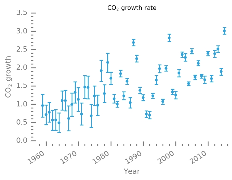
The data has a lot of spread in the middle of the range, roughly between 1980 and 2000. In one way, it looks like two lines with a jump at 1985 could be fitted. However, it is not clear why this would be the case; perhaps the two distributions of uncertainties have something to do with it?

In Scikit-learn, the learning is done by first initiating the estimator, an object where we call the fit method to train the dataset. This means that we first have to import the estimator. In this example, I will show you two different estimators and the resulting fits that they produce. The first is the simple linear model and the second is the LASSO estimator. There are many different linear models in Scikit-learn: RANSAC, Theil-Sen, and linear models based on stochastic gradient descent (SGD) learning, to name a few. After going through this example, you should look at another estimator and try it out. We first import the ones that we will work with, and also the cross_validation function, which we will use to separate the dataset into two parts—training and testing:

from sklearn.linear_model import LinearRegression, Lasso 
from sklearn import cross_validation 

As we want to be able to validate our fit and see how good it is, we do not use all of the data. We use the train_test_split function in cross_validation to put 25% of the data in a testing set and 75% in the training set. Play around with different values and see how the fit results change in the end. Then, we store the x and y values in appropriate structures. The x values have to have one extra axis. This could also be done with the x_train.reshape(-1,1) code; the way we do it here gives the same effect. We also create an array to later plot the fit with x values that we know span the whole range and a bit more:

x_test, x_train, y_test, y_train = cross_validation.train_test_split( 
    co2_gr['year'], co2_gr['rate'],  
    test_size=0.75,  
    random_state=0) 
X_train = x_train[:, np.newaxis] 
X_test = x_test[:, np.newaxis] 
line_x = np.array([1955, 2025]) 

In the training and test data split, we also make use of the random_state parameter so that the random seed is the same and we get the same division of the training and testing set by running it multiple times (for exact reproducibility). We are now ready to train the data, the first is the simple linear regression model. To run the machine learning algorithms on the training set, we first create an estimator object/class and then we simply train the model by calling the fit method with the training x and y values as input:

est_lin = LinearRegression() 
est_lin.fit(X_train, y_train) 
lin_pred = est_lin.predict(line_x.reshape(-1, 1)) 

Here, I also added a calculation of the predicted y values from the array that we created earlier, and to show an alternative way of restructuring the input array, I used the reshape method. Next is the LASSO model, and we do exactly the same, except that in creating the model object we now have the option of giving it extra parameters. The alpha parameter is basically what separates this model from the preceding simple linear regression model. If it is set to zero, the model becomes the same as the linear model. The LASSO model alpha input modifies the loss function and the default value is 1. Try different values, although 0 is not good to choose as the model is not made to operate without the added penalty to the loss function:

est_lasso = Lasso(alpha=0.7) 
est_lasso.fit(X_train, y_train) 
lasso_pred = est_lasso.predict(line_x.reshape(2, 1)) 

To see the results, we first print out the estimates of the coefficients, mean square discrepancy or error (mean squared residuals), and variance score. The variance score is a method in the Scikit-learn model (estimator) that we create. While a variance score of 1 means that it is able to predict the values perfectly, a score of 0 means that no values were predicted and there is no (linear) relationship between the variables. The coefficients are accessed with estimator.coeff_ and estimator.intercept_. To get the mean square error, we simply take the difference between the predicted and observed values, which are calculated with estimator.predict(x), where x is x values where you want to predict y values. This should be calculated on the test data and not the training set. We first create a function to calculate this and print the relevant diagnostics:

def printstuff(estimator, A, b): 
    name = estimator.__str__().split('(')[0] 
    print('+'*6, name, '+'*6) 
    print('Slope: {0:.3f} Intercept:{1:.2f} '.format( 
            estimator.coef_[0], estimator.intercept_)) 
    print("Mean squared residuals: {0:.2f}".format( 
          np.mean((estimator.predict(A) - b)**2)) )  
    print('Variance score: {0:.2f}'.format( 
            estimator.score(A, b)) ) 

With this function, we can now print the results of the fitting in a way that gives us the estimated slope and intercept, mean squared residuals, and variance score:

printstuff(est_lin, X_test, y_test) 
printstuff(est_lasso, X_test, y_test) 

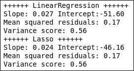
The LASSO model estimates lower values to the slope and intercept, but gives a similar mean squared residuals and variance score to the linear regression model. The spread in the data is too much to conclude whether any of them produce more reliable estimates. We can, of course, plot all of these results in a figure together with the data:

fig = plt.figure() 
ax = fig.add_subplot(111) 
ax.scatter(X_train, y_train, marker='s', 
        label='Train', color='IndianRed') 
ax.scatter(X_test, y_test, label='Test',  
        color='SteelBlue') 
ax.plot(line_x, lin_pred, color='Green', 
        label='Linreg', lw=2) 
ax.plot(line_x, lasso_pred, color='Coral', 
        dashes=(5,4), label='LASSO', lw=2) 
ax.set_xlabel('Year') 
ax.set_ylabel('CO$_2$ growth rate') 
ax.legend(loc=2, fontsize=10, numpoints=1) 
despine(ax) 
plt.minorticks_on() 
ax.locator_params(axis='x', nbins=5) 
ax.locator_params(axis='y', nbins=7) 
ax.set_xlim(1950,2030) 
ax.set_title('CO$_2$ growth rate'), 

The fits differ slightly, but are definitely within each other's uncertainty. The spread in the data points is relatively large. The squares show the training set and the circles show the testing (validation) set. Extrapolating outside this range would, however, predict significantly different values.

We can calculate the R² score, just as before with classical OLS regression:

from sklearn.metrics import r2_score 
r2_lin = r2_score(co2_gr['rate'],  
                  est_lin.predict( 
                    co2_gr['year'].reshape(-1,1))) 
r2_lasso = r2_score(co2_gr['rate'],  
                    est_lasso.predict( 
                        co2_gr['year'].reshape(-1,1))) 
print('LinearSVC: {0:.2f}
LASSO: 
	   {1:.2f}'.format(r2_lin, r2_lasso)) 

The R² values are relatively high, despite the significant spread in the data points and limited size of the data.

We will quickly make a comparison with both the statsmodels' OLS regression and Bayesian inference with a linear model. The Bayesian inference and OLS fits are the same as in Chapter 6 , Bayesian Methods, and a small version is repeated here:

import pymc 
x = co2_gr['year'].as_matrix()   
y = co2_gr['rate'].as_matrix() 
y_error = co2_gr['err'].as_matrix() 
def model(x, y):  
    slope = pymc.Normal('slope', 0.1, 1.) 
    intercept = pymc.Normal('intercept', -50., 10.) 
    @pymc.deterministic(plot=False) 
    def linear(x=x, slope=slope, intercept=intercept): 
        return x * slope + intercept 
    f = pymc.Normal('f', mu=linear, tau=1.0/y_error,                       value=y, observed=True) 
    return locals() 
MDL = pymc.MCMC(model(x,y)) 
MDL.sample(5e5, 5e4, 100) 
y_fit = MDL.stats()['linear']['mean'] 
slope = MDL.stats()['slope']['mean'] 
intercept = MDL.stats()['intercept']['mean'] 

For the OLS model, we again use the formula framework to express the relationship between our variables:

import statsmodels.formula.api as smf 
from statsmodels.sandbox.regression.predstd import wls_prediction_std 
ols_results = smf.ols("rate ~ year", co2_gr).fit() 
ols_params = np.flipud(ols_results.params) 

Now that we have the results from all three methods, let's print out the slope and intercept for them:

print('     Slope  Intercept 
ML :  
{0:.3f} {1:.3f} 
OLS: {2:.3f}  
{3:.3f} 
Bay: {4:.3f}  
{5:.3f}'.format(est_lin.coef_[0], est_lin.intercept_, 
                ols_params[0],ols_params[1], 
                slope, intercept) ) 

While the overall results are similar, Bayesian inference seems to estimate absolute values that are lower than the other methods. We can now visualize these different estimates together with the data:

fig = plt.figure() 
ax = fig.add_subplot(111) 
ax.errorbar(x, y, yerr=y_error, ls='None',   
        elinewidth=1.5, capthick=1.5, 
        marker='.', ms=8, label='Observed') 
ax.set_xlabel('Year') 
ax.set_ylabel('CO$_2$ growth rate') 
ax.plot([x.min(), x.max()],  
        [ols_results.fittedvalues.min(),  
         ols_results.fittedvalues.max()],  
        lw=1.5, label='OLS', 
        dashes=(13,5)) 
ax.plot(x, y_fit, lw=1.5, 
        label='pymc') 
ax.plot([x.min(), x.max()],  
        est_lin.predict([[x.min(), ], [x.max(), ]]), 
        label='Scikit-learn', lw=1.5) 
despine(ax) 
ax.locator_params(axis='x', nbins=7) 
ax.locator_params(axis='y', nbins=4) 
ax.set_xlim((1955,2018)) 
ax.legend(loc=2, numpoints=1) 
ax.set_title('CO$_2$ growth rate'), 

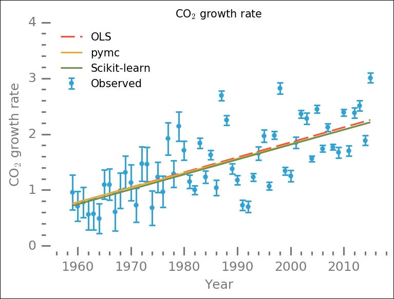
This might look like a very small difference; however, if we use these different results to extrapolate 30, 50, or even 100 years into the future, these will yield significantly different results. This example shows you how simple it is to try out different methods and models in Scikit-learn. It is also possible to create your own. Next up, we will look at one cluster identification model in Scikit-learn, DBSCAN.