
The matplotlib library allows configuration via the matplotlibrc files and Python code. The last option is what we are going to do in this recipe. Small configuration tweaks should not matter if your data analysis is strong. However, it doesn't hurt to have consistent and attractive plots. Another option is to apply stylesheets, which are files comparable to the matplotlibrc files. However, in my opinion, the best option is to use Seaborn on top of matplotlib. I will discuss Seaborn and matplotlib in more detail in Chapter 2, Creating Attractive Data Visualizations.
You need to install matplotlib for this recipe. Visit http://matplotlib.org/users/installing.html (retrieved July 2015) for more information. I have matplotlib 1.4.3 via Anaconda. Install Seaborn using Anaconda:
$ conda install seaborn
I have installed Seaborn 0.6.0 via Anaconda.
We can set options via a dictionary-like variable. The following function from the options.py file in dautil sets three options:
def set_mpl_options():
    mpl.rcParams['legend.fancybox'] = True
    mpl.rcParams['legend.shadow'] = True
    mpl.rcParams['legend.framealpha'] = 0.7
The first three options have to do with legends. The first option specifies rounded corners for the legend, the second options enables showing a shadow, and the third option makes the legend slightly transparent. The matplotlib rcdefaults() function resets the configuration.
To demonstrate these options, let's use sample data made available by matplotlib. The imports are as follows:
import matplotlib.cbook as cbook
import pandas as pd
import matplotlib.pyplot as plt
from dautil import options
import matplotlib as mpl
from dautil import plotting
import seaborn as sns
The data is in a CSV file and contains stock price data for AAPL. Use the following commands to read the data and stores them in a pandas DataFrame:
data = cbook.get_sample_data('aapl.csv', asfileobj=True)
df = pd.read_csv(data, parse_dates=True, index_col=0)
Resample the data to average monthly values as follows:
df = df.resample('M')The full code is in the configure_matplotlib.ipynb file in this book's code bundle:
import matplotlib.cbook as cbook
import pandas as pd
import matplotlib.pyplot as plt
from dautil import options
import matplotlib as mpl
from dautil import plotting
import seaborn as sns


data = cbook.get_sample_data('aapl.csv', asfileobj=True)
df = pd.read_csv(data, parse_dates=True, index_col=0)
df = df.resample('M')
close = df['Close'].values
dates = df.index.values
fig, axes = plt.subplots(4)


def plot(title, ax):
    ax.set_title(title)
    ax.set_xlabel('Date')

    plotter = plotting.CyclePlotter(ax)
    plotter.plot(dates, close, label='Close')
    plotter.plot(dates, 0.75 * close, label='0.75 * Close')
    plotter.plot(dates, 1.25 * close, label='1.25 * Close')

    ax.set_ylabel('Price ($)')
    ax.legend(loc='best')

plot('Initial', axes[0])
sns.reset_orig()
options.set_mpl_options()

plot('After setting options', axes[1])

sns.reset_defaults()
plot('After resetting options', axes[2])

with plt.style.context(('dark_background')):
    plot('With dark_background stylesheet', axes[3])
    fig.autofmt_xdate()
    plt.show()
The program plots the data and arbitrary upper and lower band with the default options, custom options, and after a reset of the options. I used the following helper class from the plotting.py file of dautil:
from itertools import cycle


class CyclePlotter():
    def __init__(self, ax):
        self.STYLES = cycle(["-", "--", "-.", ":"])
        self.LW = cycle([1, 2])
        self.ax = ax

    def plot(self, x, y, *args, **kwargs):
        self.ax.plot(x, y, next(self.STYLES),
                     lw=next(self.LW), *args, **kwargs)
The class cycles through different line styles and line widths. Refer to the following plot for the end result:
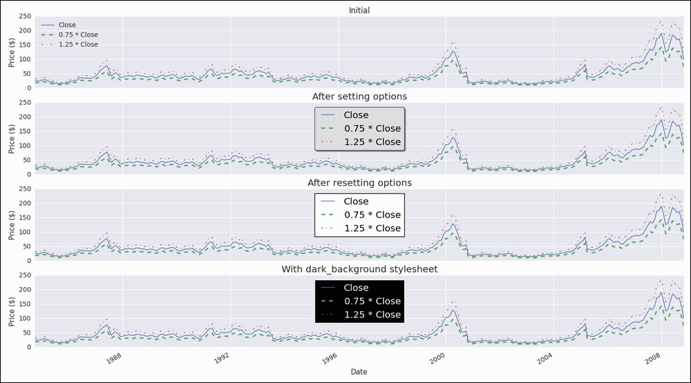
Importing Seaborn dramatically changes the look and feel of matplotlib plots. Just temporarily comment the seaborn lines out to convince yourself. However, Seaborn doesn't seem to play nicely with the matplotlib options we set, unless we use the Seaborn functions reset_orig() and reset_defaults().
- The matplotlib customization documentation at http://matplotlib.org/users/customizing.html (retrieved July 2015)
- The matplotlib documentation about stylesheets at http://matplotlib.org/users/style_sheets.html (retrieved July 2015)