
In the previous recipe, Setting up Spark, we covered a basic setup of Spark. If you followed the Using HDFS recipe, you can optionally serve the data from Hadoop. In this case, you need to specify the URL of the file in this manner, hdfs://hdfs-host:port/path/direct_marketing.csv.
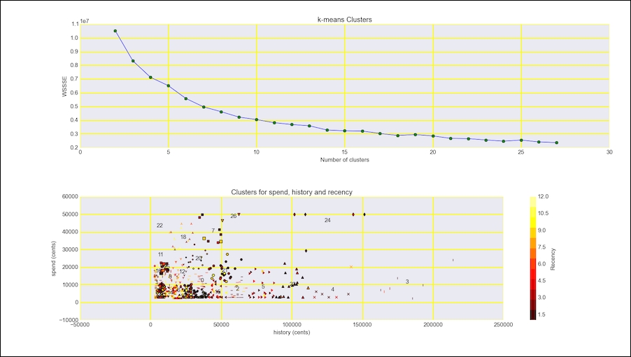
We will use the same data as we did in the Implementing a star schema with fact and dimension tables recipe. However, this time we will use the spend, history, and recency columns. The first column corresponds to recent purchase amounts after a direct marketing campaign, the second to historical purchase amounts, and the third column to the recency of purchase in months. The data is described in http://blog.minethatdata.com/2008/03/minethatdata-e-mail-analytics-and-data.html (retrieved September 2015). We will apply the popular K-means machine-learning algorithm to cluster the data. Chapter 9, Ensemble Learning and Dimensionality Reduction, pays more attention to machine learning algorithms. The K-means algorithm attempts to find the best clusters for a dataset given a number of clusters. We are supposed to either know this number or find it through trial and error. In this recipe, I evaluate the clusters through the Within Set Sum Squared Error (WSSSE), also known as Within Cluster Sum of Squares (WCSS). This metric calculates the sum of the squared error of the distance between each point and its assigned cluster. You can read more about evaluation metrics in Chapter 10, Evaluating Classifiers, Regressors, and Clusters.
The code for this recipe is in the clustering_spark.py file in this book's code bundle:
- The imports are as follows:
from pyspark.mllib.clustering import KMeans
from pyspark import SparkContext
import dautil as dl
import csv
import matplotlib.pyplot as plt
import matplotlib as mpl
from matplotlib.colors import Normalize
- Define the following function to compute the error:
def error(point, clusters): center = clusters.centers[clusters.predict(point)] return dl.stats.wssse(point, center) - Read and parse the data, as follows:
sc = SparkContext() csv_file = dl.data.get_direct_marketing_csv() lines = sc.textFile(csv_file) header = lines.first().split(',') cols_set = set(['recency', 'history', 'spend']) select_cols = [i for i, col in enumerate(header) if col in cols_set] - Set up the following RDDs:
header_rdd = lines.filter(lambda l: 'recency' in l) noheader_rdd = lines.subtract(header_rdd) temp = noheader_rdd.map(lambda v: list(csv.reader([v]))[0]) .map(lambda p: (int(p[select_cols[0]]), dl.data.centify(p[select_cols[1]]), dl.data.centify(p[select_cols[2]]))) # spend > 0 temp = temp.filter(lambda x: x[2] > 0) - Cluster the data with the k-means algorithm:
points = [] clusters = None for i in range(2, 28): clusters = KMeans.train(temp, i, maxIterations=10, runs=10, initializationMode="random") val = temp.map(lambda point: error(point, clusters)) .reduce(lambda x, y: x + y) points.append((i, val)) - Plot the clusters, as follows:
dl.options.mimic_seaborn()
fig, [ax, ax2] = plt.subplots(2, 1)
ax.set_title('k-means Clusters')
ax.set_xlabel('Number of clusters')
ax.set_ylabel('WSSSE')
dl.plotting.plot_points(ax, points)

collected = temp.collect()
recency, history, spend = zip(*collected)
indices = [clusters.predict(c) for c in collected]
ax2.set_title('Clusters for spend, history and recency')
ax2.set_xlabel('history (cents)')
ax2.set_ylabel('spend (cents)')
markers = dl.plotting.map_markers(indices)
colors = dl.plotting.sample_hex_cmap(name='hot', ncolors=len(set(recency)))

for h, s, r, m in zip(history, spend, recency, markers):
    ax2.scatter(h, s, s=20 + r, marker=m, c=colors[r-1])

cma = mpl.colors.ListedColormap(colors, name='from_list', N=None)
norm = Normalize(min(recency), max(recency))
msm = mpl.cm.ScalarMappable(cmap=cma, norm=norm)
msm.set_array([])
fig.colorbar(msm, label='Recency')

for i, center in enumerate(clusters.clusterCenters):
    recency, history, spend = center
    ax2.text(history, spend, str(i))

plt.tight_layout()
plt.show()
Refer to the following screenshot for the end result (the numbers in the plot correspond to cluster centers):
K-means clustering assigns data points to k clusters. The problem of clustering is not solvable directly, but we can apply heuristics, which achieve an acceptable result. The algorithm for k-means iterates between two steps not including the (usually random) initialization of k-means:
The algorithm stops when the cluster assignments become stable.
Spark 1.5.0 added experimental support to stream K-means. Due to the experimental nature of these new features, I decided to not discuss them in detail. I have added the following example code in the streaming_clustering.py file in this book's code bundle:
import dautil as dl
from pyspark.mllib.clustering import StreamingKMeansModel
from pyspark import SparkContext

csv_file = dl.data.get_direct_marketing_csv()
csv_rows = dl.data.read_csv(csv_file)

stkm = StreamingKMeansModel(28 * [[0., 0., 0.]], 28 * [1.])
sc = SparkContext()

for row in csv_rows:
    spend = dl.data.centify(row['spend'])

    if spend > 0:
        history = dl.data.centify(row['history'])
        data = sc.parallelize([[int(row['recency']),
                               history, spend]])
        stkm = stkm.update(data, 0., 'points')

print(stkm.centers)- Building Machine Learning Systems with Python, Willi Richert, and Luis Pedro Coelho (2013)
- The Wikipedia page about K-means clustering is at https://en.wikipedia.org/wiki/K-means_clustering (retrieved September 2015)