
It is sometimes useful to imagine that the data we observe is just the tip of an iceberg. If you get into this mindset, then you probably will want to know how big this iceberg actually is. Obviously, if you can't see the whole thing, you can still try to extrapolate from the data you have. In statistics we try to estimate confidence intervals, which are an estimated range usually associated with a certain confidence level quoted in percentages.
The scipy.stats.bayes_mvs() function estimates confidence intervals for mean, variance, and standard deviation. The function uses Bayesian statistics to estimate confidence assuming that the data is independent and normally distributed. Jackknifing is an alternative deterministic algorithm to estimate confidence intervals. It falls under the family of resampling algorithms. Usually, we generate new datasets under the jackknifing algorithm by deleting one value (we can also delete two or more values). We generate data N times, where N is the number of values in the dataset. Typically, if we want a 5 percent confidence level, we estimate the means or variances for the new datasets and determine the 2.5 and 97.5 percentile values.
In this recipe, we estimate confidence intervals with the scipy.stats.bayes_mvs() function and jackknifing:
- The imports are as follows:
from scipy import stats
import dautil as dl
from dautil.stats import jackknife
import pandas as pd
import matplotlib.pyplot as plt
import numpy as np
from IPython.html.widgets.interaction import interact
from IPython.display import HTML
- Define the following function to visualize the Scipy result using error bars:
def plot_bayes(ax, metric, var, df): vals = np.array([[v.statistic, v.minmax[0], v.minmax[1]] for v in df[metric].values]) ax.set_title('Bayes {}'.format(metric)) ax.errorbar(np.arange(len(vals)), vals.T[0], yerr=(vals.T[1], vals.T[2])) set_labels(ax, var) - Define the following function to visualize the jackknifing result using error bars:
def plot_jackknife(ax, metric, func, var, df): vals = df.apply(lambda x: jackknife(x, func, alpha=0.95)) vals = np.array([[v[0], v[1], v[2]] for v in vals.values]) ax.set_title('Jackknife {}'.format(metric)) ax.errorbar(np.arange(len(vals)), vals.T[0], yerr=(vals.T[1], vals.T[2])) set_labels(ax, var) - Define the following function, which will be called with the help of an IPython interactive widget:
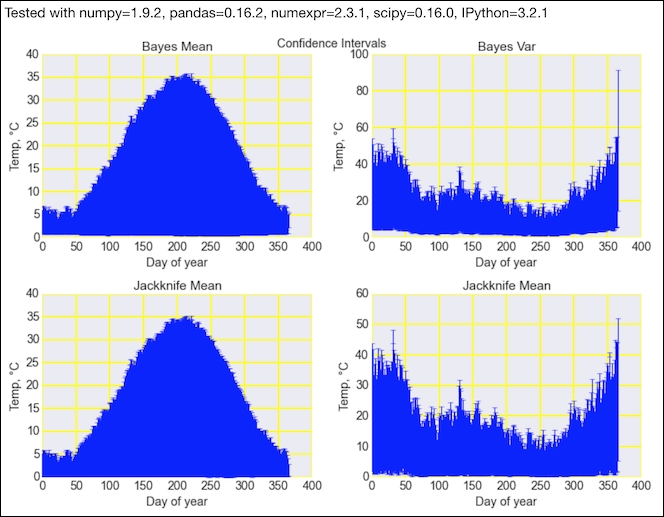
def confidence_interval(var='TEMP'): df = dl.data.Weather.load().dropna() df = dl.ts.groupby_yday(df) def f(x): return stats.bayes_mvs(x, alpha=0.95) bayes_df = pd.DataFrame([[v[0], v[1], v[2]] for v in df[var].apply(f).values], columns=['Mean', 'Var', 'Std']) fig, axes = plt.subplots(2, 2) fig.suptitle('Confidence Intervals') plot_bayes(axes[0][0], 'Mean', var, bayes_df) plot_bayes(axes[0][1], 'Var', var, bayes_df) plot_jackknife(axes[1][0], 'Mean', np.mean, var, df[var]) plot_jackknife(axes[1][1], 'Mean', np.var, var, df[var]) plt.tight_layout() - Set up an interactive IPython widget:
interact(confidence_interval, var=dl.data.Weather.get_headers())
HTML(dl.report.HTMLBuilder().watermark())
Refer to the following screenshot for the end result (see the bayes_confidence.ipynb file in this book's code bundle):
- The Wikipedia page on jackknife resampling at https://en.wikipedia.org/wiki/Jackknife_resampling (retrieved August 2015)
- T.E. Oliphant, "A Bayesian perspective on estimating mean, variance, and standard-deviation from data" (http://hdl.handle.net/1877/438, 2006)