
Cohen's kappa measures the agreement between target and predicted class similar to accuracy, but it also takes into account random chance of getting the predictions. Cohen's kappa is given by the following equation:

In this equation, p0 is the relative observed agreement and pe is the random chance of agreement derived from the data. Kappa varies between negative values and one with the following rough categorization from Landis and Koch:
- Poor agreement: kappa < 0
- Slight agreement: kappa = 0 to 0.2
- Fair agreement: kappa = 0.21 to 0.4
- Moderate agreement: kappa = 0.41 to 0.6
- Good agreement: kappa = 0.61 to 0.8
- Very good agreement: kappa = 0.81 to 1.0
I know of two other schemes to grade kappa, so these numbers are not set in stone. I think we can agree not to accept kappa less than 0.2. The most appropriate use case is, of course, to rank models. There are other variations of Cohen's kappa, but as of November 2015, they were not implemented in scikit-learn. scikit-learn 0.17 has added support for Cohen's kappa via the cohen_kappa_score() function.
- The imports are as follows:
import dautil as dl
from sklearn import metrics
import numpy as np
import ch10util
from IPython.display import HTML
- Compute accuracy, precision, recall, F1-score, and kappa for the rain predictors:
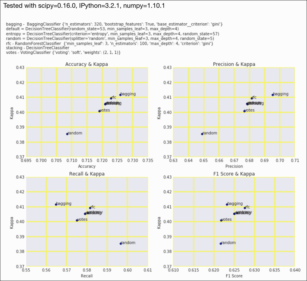
y_test = np.load('rain_y_test.npy') accuracies = [metrics.accuracy_score(y_test, preds) for preds in ch10util.rain_preds()] precisions = [metrics.precision_score(y_test, preds) for preds in ch10util.rain_preds()] recalls = [metrics.recall_score(y_test, preds) for preds in ch10util.rain_preds()] f1s = [metrics.f1_score(y_test, preds) for preds in ch10util.rain_preds()] kappas = [metrics.cohen_kappa_score(y_test, preds) for preds in ch10util.rain_preds()] - Scatter plot the metrics against kappa as follows:
sp = dl.plotting.Subplotter(2, 2, context)
dl.plotting.plot_text(sp.ax, accuracies, kappas,
                      ch10util.rain_labels(), add_scatter=True)
sp.label()

dl.plotting.plot_text(sp.next_ax(), precisions, kappas,
                      ch10util.rain_labels(), add_scatter=True)
sp.label()

dl.plotting.plot_text(sp.next_ax(), recalls, kappas,
                      ch10util.rain_labels(), add_scatter=True)
sp.label()

dl.plotting.plot_text(sp.next_ax(), f1s, kappas,
                      ch10util.rain_labels(), add_scatter=True)
sp.label()
sp.fig.text(0, 1, ch10util.classifiers())
HTML(sp.exit())
Refer to the following screenshot for the end result:
The code is in the kappa.ipynb file in this book's code bundle.
From the first two plots, we can conclude that the bagging classifier has the highest accuracy, precision, and kappa. All the classifiers have a kappa above 0.2, so they are at least somewhat acceptable.
- The Wikipedia page about Cohen's kappa at https://en.wikipedia.org/wiki/Cohen's_kappa (retrieved November 2015)