
The discrete wavelet transform (DWT) captures information in both the time and frequency domains. The mathematician Alfred Haar created the first wavelet. We will use this Haar wavelet in this recipe too. The transform returns approximation and detail coefficients, which we need to use together to get the original signal back. The approximation coefficients are the result of a low-pass filter. A high-pass filter produces the detail coefficients. The Haar wavelet algorithm is of order O(n) and, similar to the STFT algorithm (refer to the Analyzing the frequency spectrum of audio recipe), combines frequency and time information.
The difference with the Fourier transform is that we express the signal as a sum of sine and cosine terms, while the wavelet is represented by a single wave (wavelet function). Just as in the STFT, we split the signal in the time domain and then apply the wavelet function to each segment. The DWT can have multiple levels in this recipe, we don't go further than the first level. To obtain the next level, we apply the wavelet to the approximation coefficients of the previous level. This means that we can have multiple level detail coefficients.
As the dataset, we will have a look at the famous Nile river flow, which even the Greek historian Herodotus wrote about. More recently, in the previous century, the hydrologist Hurst discovered a power law for the rescaled range of the Nile river flow in the year. Refer to the See also section for more information. The rescaled range is not difficult to compute, but there are lots of steps as described in the following equations:

The Hurst exponent from the power law is an indicator of trends. We can also get the Hurst exponent with a more efficient procedure from the wavelet coefficients.
Install pywavelets, as follows:
$ pip install pywavelets
I used pywavelets 0.3.0 for this recipe.
- The imports are as follows:
from statsmodels import datasets
import matplotlib.pyplot as plt
import pywt
import pandas as pd
import dautil as dl
import numpy as np
import seaborn as sns
import warnings
from IPython.display import HTML
- Filter warnings as follows (optional step):
warnings.filterwarnings(action='ignore', message='.*Mean of empty slice.*') warnings.filterwarnings(action='ignore', message='.*Degrees of freedom <= 0 for slice.*') - Define the following function to calculate the rescaled range:
def calc_rescaled_range(X): N = len(X) # 1. Mean mean = X.mean() # 2. Y mean adjusted Y = X - mean # 3. Z cumulative deviates Z = np.array([Y[:i].sum() for i in range(N)]) # 4. Range R R = np.array([0] + [np.ptp(Z[:i]) for i in range(1, N)]) # 5. Standard deviation S S = np.array([X[:i].std() for i in range(N)]) # 6. Average partial R/S return [np.nanmean(R[:i]/S[:i]) for i in range(N)] - Load the data and transform it with a Haar wavelet:
data = datasets.get_rdataset('Nile', cache=True).data cA, cD = pywt.dwt(data['Nile'].values, 'haar') coeff = pd.DataFrame({'cA': cA, 'cD': cD}) - Plot the Nile river flow as follows:
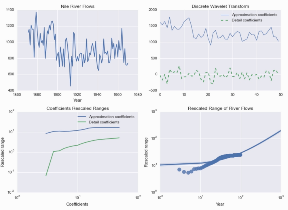
sp = dl.plotting.Subplotter(2, 2, context)
sp.ax.plot(data['time'], data['Nile'])
sp.label()
- Plot the approximation and detail coefficients of the transformed data:
cp = dl.plotting.CyclePlotter(sp.next_ax())
cp.plot(range(len(cA)), cA, label='Approximation coefficients')
cp.plot(range(len(cD)), cD, label='Detail coefficients')
sp.label()
- Plot the rescaled ranges of the coefficients as follows:
sp.next_ax().loglog(range(len(cA)), calc_rescaled_range(cA), label='Approximation coefficients') sp.ax.loglog(range(len(cD)), calc_rescaled_range(cD), label='Detail coefficients') sp.label() - Plot the rescaled ranges of the Nile river flow data with a fit:
range_df = pd.DataFrame(data={'Year': data.index,
                              'Rescaled range':
                              calc_rescaled_range(data['Nile'])})
sp.next_ax().set(xscale="log", yscale="log")
sns.regplot('Year', 'Rescaled range', range_df, ax=sp.ax, order=1,
            scatter_kws={"s": 100})
sp.label()
HTML(sp.exit())
Refer to the following screenshot for the end result:
The relevant code is in the discrete_wavelet.ipynb file in this book's code bundle.
- The Wikipedia page about the discrete wavelet transform at https://en.wikipedia.org/wiki/Discrete_wavelet_transform (retrieved September 2015)
- The Wikipedia page about the rescaled range at https://en.wikipedia.org/wiki/Rescaled_range (retrieved September 2015)
- The Wikipedia page about the Hurst exponent at https://en.wikipedia.org/wiki/Hurst_exponent (retrieved September 2015)