
Many aspects of smoothing are comparable to regression; therefore, you can apply some of the techniques in Chapter 10, Evaluating Classifiers, Regressors, and Clusters, to smoothing too. In this recipe, we will smooth with the Savitzky-Golay filter, which conforms to the following equation:

The filter fits points within a rolling window of size n to a polynomial of order m. Abraham Savitzky and Marcel J. E. Golay created the algorithm around 1964 and first applied it to chemistry problems. The filter has two parameters that naturally form a grid. As in regression problems, we will take a look at a difference, in this case, the difference between the original signal and the smoothed signal. We assume, just like when we fit data, that the residuals are random and follow a Gaussian distribution.
The following steps are from the eval_smooth.ipynb file in this book's code bundle:
- The imports are as follows:
import dautil as dl
import matplotlib.pyplot as plt
from scipy.signal import savgol_filter
import pandas as pd
import numpy as np
import seaborn as sns
from IPython.display import HTML
- Define the following helper functions:
def error(data, fit): return data - fit def win_rng(): return range(3, 25, 2) def calc_mape(i, j, pres): return dl.stats.mape(pres, savgol_filter(pres, i, j)) - Load the atmospheric pressure data as follows:
pres = dl.data.Weather.load()['PRESSURE'].dropna() pres = pres.resample('A') - Plot the original data and the filter with window size 11 and various polynomial orders:
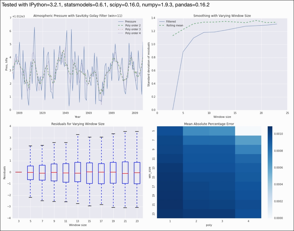
sp = dl.plotting.Subplotter(2, 2, context) cp = dl.plotting.CyclePlotter(sp.ax) cp.plot(pres.index, pres, label='Pressure') cp.plot(pres.index, savgol_filter(pres, 11, 2), label='Poly order 2') cp.plot(pres.index, savgol_filter(pres, 11, 3), label='Poly order 3') cp.plot(pres.index, savgol_filter(pres, 11, 4), label='Poly order 4') sp.label(ylabel_params=dl.data.Weather.get_header('PRESSURE')) - Plot the standard deviations of the filter residuals for varying window sizes:
cp = dl.plotting.CyclePlotter(sp.next_ax()) stds = [error(pres, savgol_filter(pres, i, 2)).std() for i in win_rng()] cp.plot(win_rng(), stds, label='Filtered') stds = [error(pres, pd.rolling_mean(pres, i)).std() for i in win_rng()] cp.plot(win_rng(), stds, label='Rolling mean') sp.label() - Plot the box plots of the filter residuals:
sp.label(advance=True) sp.ax.boxplot([error(pres, savgol_filter(pres, i, 2)) for i in win_rng()]) sp.ax.set_xticklabels(win_rng()) - Plot the MAPE for a grid of window sizes and polynomial orders:
sp.label(advance=True)
df = dl.report.map_grid(win_rng()[1:], range(1, 5),
                 ['win_size', 'poly', 'mape'], calc_mape, pres)
sns.heatmap(df, cmap='Blues', ax=sp.ax)
HTML(sp.exit())
Refer to the following screenshot for the end result:
- The Wikipedia page about the Savitzky-Golay filter at https://en.wikipedia.org/wiki/Savitzky%E2%80%93Golay_filter (retrieved September 2015)
- The
savgol_filter()function documented at https://docs.scipy.org/doc/scipy/reference/generated/scipy.signal.savgol_filter.html (retrieved September 2015)