The main reason that we emphasize the cumulative distribution function is because, once we have access to it, we can compute any probabilities associated with the model. This is because the cdf is a universal way to specify a random variable. In particular, there is no distinction between the descriptions for continuous or discrete data. The density function of a random variable is also an important concept so we will present it in the next section. In this section, we will see how to use the cdf to do computations related to a random variable.

The functions that we will use with distributions are part of SciPy and contained in the scipy.stats module, which we import with the following code:

import scipy.stats as st 

After this, we can refer to functions in the package with the abbreviation st.

This module contains a large number of predefined distributions, and we encourage you to visit the official documentation at http://docs.scipy.org/doc/scipy/reference/stats.html to see what is available. Fortunately for us, the module is organized in such a way that all distributions are handled in a uniform way, as shown in the following line:

st.<rv_name>.<function>(<arguments>) 

The components of this expression are as follows:

The following table lists some of the functions that are available for each random variable:

Whenever we specify a distribution, we need to set the parameters that characterize the random variable of interest. Most models have, at least, a location and scale, which are commonly referred to as the shape parameters of the random variable. The location specifies a shift in the distribution and the scale represents a rescaling of the values (such as when units are changed).

In the following example, we will concentrate on Normal distribution as this is certainly an important case. However, you should be aware that the computation patterns we present can be used with any distribution. So, if one needs, for example, to work with a Log-Laplace distribution, all they have to do is replace norm in the following examples with loglaplace. Of course, it is necessary to consult the documentation to make sure that the correct parameters are being used for the distribution of interest.

For a Normal distribution, the location parameter gives the mean of the distribution and the scale represents the standard deviation of the distribution. These terms will be defined later in the chapter, but they are numbers that measure the center and spread of the distribution. To give a concrete example of a normally distributed random variable, let's consider the height of women over 20 years of age, as in National Health Statistics Reports, Number 10, October 2008, available online at  http://www.cdc.gov/nchs/data/nhsr/nhsr010.pdf . This report contains anthropometric reference data for the U.S. population, according to age group. On page 14, the height of women over 20 is reported as having a mean of 63.8 inches with a standard error of 0.06. The sample size is 4,857.

We will assume that heights are normally distributed (which, as it happens, is a reasonable assumption). To characterize the distribution, we need the mean and standard deviation. The mean is given directly in the report. The standard deviation is not reported directly but can be computed from the standard error and sample size, according to the following formula:

The standard error is a measure of sample variability that will be introduced in Chapter 4, Regression. We are also ignoring the issue that we are using the sampl e standard deviation instead of the population standard deviation, but the sample is large enough to justify this approach, as will be seen in Chapter 4, Regression. We start by defining the distribution to be used as the model for this situation, using the following code:

N = 4857 
mean = 63.8 
serror = 0.06 
sdev = serror * np.sqrt(N) 
rvnorm = st.norm(loc=mean, scale=sdev) 

In this code, we first define variables to represent the sample size, mean, and standard error. Then, the standard deviation is computed according to the preceding formula. In the last line of code, we call the norm() function, passing the mean and standard deviation as parameters. The object returned by the function is assigned to the rvnorm variable, and it is through this variable that we access the functionality of the package.

A good place to start with any distribution is to make graphs so that we can have an idea of the shape of the distribution. This can be accomplished with the following code:

xmin = mean-3*sdev 
xmax = mean+3*sdev 
xx = np.linspace(xmin,xmax,200) 
plt.figure(figsize=(8,3)) 
plt.subplot(1,2,1) 
plt.plot(xx, rvnorm.cdf(xx)) 
plt.title('Cumulative distribution function') 
plt.xlabel('Height (in)') 
plt.ylabel('Proportion of women') 
plt.axis([xmin, xmax, 0.0, 1.0]) 
plt.subplot(1,2,2) 
plt.plot(xx, rvnorm.pdf(xx)) 
plt.title('Probability density function') 
plt.xlabel('Height (in)') 
plt.axis([xmin, xmax, 0.0, 0.1]); 

Most of the lines of the preceding code deal with setting up and formatting the plot. The two most important pieces of code are the two calls to the plot() function. The first call is as follows:

plt.plot(xx, rvnorm.cdf(xx)) 

The xx array was previously defined to contain the x coordinates to be plotted. The rvnorm.cdf(xx) function call computes the value of the cdf. The second call is analogous as follows:

plt.plot(xx, rvnorm.pdf(xx)) 

The only difference is that now we call rvnorm.pdf(xx) to compute the probability density function. The overall effect of the code is to generate side-by-side plots of the cdf and density function. These are the familiar S-shaped and bell-shaped curves, which are characteristic of a Normal distribution:

Let's now see how we can use the cdf to compute quantities related to the distribution. Suppose that a garment factory uses a classification of women's heights, as indicated in the following table:

What percentage of women are in the Average category? We can get this information directly from the cdf. Recall that this function gives the proportion of data values up to a given value. So, the proportion of women with heights up to 68 inches is computed by the following expression:

rvnorm.cdf(68) 

Likewise, the proportion of women with heights up to 63 inches is computed with the following expression:

rvnorm.cdf(63) 

The proportion of women with heights between 63 inches and 68 inches is the difference between these values. As we want a percentage, we have to multiply the result by 100, as shown in the following line of code:

100 * (rvnorm.cdf(68) - rvnorm.cdf(63)) 

The result of this computation shows that approximately 42.8% of women are Average according to this classification. To compute the percentages for the three categories and display them in a nice format, we can use the following code:

categories = [ 
    ('Petite', 59, 63), 
    ('Average', 63, 68), 
    ('Tall', 68, 71), 
    ] 
for cat, vmin, vmax in categories: 
    percent = 100 * (rvnorm.cdf(vmax) - rvnorm.cdf(vmin)) 
    print('{:>8s}: {:.2f}'.format(cat, percent)) 

In this code segment, we start by creating a Python list that describes the categories. Each category is represented by a three-element tuple, containing the category name, minimum height, and maximum height. We then use a for loop to iterate over the categories. For each category, we first compute the percentage of women in the category using the cdf, and then print the result.

A somewhat unexpected feature of this classification is that it imposes the lowest and highest values on women's heights. We can compute the percentage of women that are too short or too tall to fit in any of the categories with the following code:

too_short = 100 * rvnorm.cdf(59) 
too_tall = 100 * (1 - rvnorm.cdf(71)) 
unclassified = too_short + too_tall 
print(too_short, too_tall, unclassified) 

Running this code, we conclude that almost 17% of the women are unclassified! This may not seem too much, but any sector of industry that neglects such a portion of its customer base will be losing profits. Suppose that we have been hired to come up with a more effective classification. Let's say that we agree that 50% of women at the center of the distribution should be classified as Average, the top 25% should be considered Tall, and the lower 25% should be considered Petite. In other words, we want to use the quartiles of the distribution to define height categories. Notice that this is an arbitrary decision and may not be realistic.

We can find the threshold values between the categories using the inverse of the cdf. This is computed by the ppf() method, which stands for percent point function. This is shown in the following code:

a = rvnorm.ppf(0.25) 
b = rvnorm.ppf(0.75) 
print(a, b) 

From the preceding computation, it follows that, according to our criterion, women should be considered Average if their heights are between approximately 61 inches and 67 inches. It seems that the original classification is skewed toward taller women (there is a large proportion of short women that do not fit the classification). We can only speculate why this is the case. Industry standards are sometimes inherited from tradition and may have been set without regard to actual data.

It is worthy to notice that, in all the computations we did, we used the cumulative distribution function and not the probability density function, which we will present in the next section. Indeed, this will be the case with most computations that are needed in inference. The fact that most people prefer to use probability densities when defining distributions may simply be due to historical bias. In fact, both views of a random variable are important and find a place in theory and applications.

To finish this example, let's compute some relevant parameters (that is, point estimates) for the distribution of heights using the following code:

mean, variance, skew, kurtosis = rvnorm.stats(moments='mvks') 
print(mean, variance, skew, kurtosis) 

This will print values of 63.8 for the mean, 17.4852 for the variance, and 0 for both skew and kurtosis. These values are interpreted as follows:

For our next example, let's suppose that we need to build a simulation for the time-to-failure of some equipment. A frequently used model for this situation is the Weibull distribution, named after Waloddi Weibull, who carefully studied the distribution in 1951. This distribution is described in terms of two numbers called the scale parameter, denoted by η (eta) and the shape parameter, denoted by β (beta). Both parameters must be positive numbers.

The shape parameter is related to how the failure rate of the equipment depends on its age (or operation time) as follows:

The scale parameter, on the other hand, determines how much the distribution spreads. Put in an intuitive way, a larger value of the scale parameter corresponds to more uncertainty regarding predictions for the failure time. Notice that, in this case, the scale parameter cannot be interpreted as the standard deviation of the model.

Let's say that we want to simulate a Weibull distribution with the shape parameter βpara and scale parameter ηand. You are encouraged, at this point, to generate plots of the cumulative distribution and probability density functions for the Weibull distribution by modifying the code that we previously used for the Normal distribution. To create the distribution, the following code can be used:

eta = 1.0 
beta = 1.5 
rvweib = st.weibull_min(beta, scale=eta) 

After defining the eta and beta parameters, we call the weibull_min() function, which generates the appropriate object. After producing the graphs, you will notice that the Weibull distribution is markedly asymmetric, having a long right tail after peaking.

Let's now get back to the problem of simulating the distribution. To produce a sample of size 500 following a Weibull distribution, we use the following code:

weib_variates = rvweib.rvs(size=500) 
print(weib_variates[:10]) 

In this code, we simply call the rvs() method, passing the desired sample size as an argument. The abbreviation rvs stands for random variates. As the generated sample is quite large, we simply print the first 10 values. We can use a histogram to visualize the sample, as shown in the following code:

weib_df = DataFrame(weib_variates,columns=['weibull_variate']) 
weib_df.hist(bins=30); 

In this code, we first convert the data to a Pandas DataFrame object as we want to use Pandas' plotting capabilities. Then, we simply call the hist() method, passing the number of bins as an argument. This results in the following histogram:

Notice the peak around 0.5 followed by a decaying tail toward the right. Also notice the few values at the extreme right of the histogram. These represent survival times that are large compared with the bulk of the data.

Finally, we want to assess how good the simulation is. To this end, we can plot the cumulative distribution function of the sample, compared with that of the theoretical distribution. This is achieved with the following code:

xmin = 0 
xmax = 3.5 
xx = np.linspace(xmin,xmax,200) 
plt.plot(xx, rvweib.cdf(xx), color='orange', lw=5) 
plot_cdf(weib_variates, plot_range=[xmin, xmax], scale_to=1, lw=2, color='green') 
plt.axis([xmin, xmax, 0, 1]) 
plt.title('Weibul distribution simulation', fontsize=14) 
plt.xlabel('Failure Time', fontsize=12); 

This code is essentially a combination of code segments that we have seen before. We call the plot() function with appropriate arguments to generate a plot of the theoretical cdf, and then use the plot_cdf() function, previously defined in this chapter, to plot the cdf of the data. It is seen that the two curves show pretty good agreement.

As a final example in this section, let's explore the fit() method, which attempts to fit a distribution to the data. Let's go back to the dataset with wing lengths of houseflies. As previously stated, we suspect that the data is normally distributed. We can find the Normal distribution that best fits the data with the following code:

wing_lengths = np.fromfile('data/housefly-wing-lengths.txt', 
                           sep='
', dtype=np.int64) 
mean, std = st.norm.fit(wing_lengths) 
print(mean, std) 

Just to be on the safe side, we read the data again using the fromfile() function. We then use the st.norm.fit() function to fit a Normal distribution to the dataset. The fit() function returns the mean and standard deviation of the fitted Normal distribution. This is an example of parameter estimation (point estimate). The next question is: how good is the fit? We can evaluate this graphically by generating a quantile plot, as shown in  Chapter 2 , Exploring Data. The following is the code:

st.probplot(wing_lengths, dist='norm', plot=plt) 
plt.grid(lw=1.5, lw='dashed'), 

This code will produce the following plot:

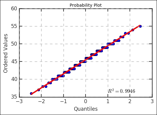
Notice that the sample falls very close to a straight line, indicating that a Normal distribution is a good fit for this data. Notice, however, that there is some clustering in the data, which is a consequence of repeated values (measurement imprecision and rounding).

We finalize this section by encouraging you to visit the SciPy documentation for the stats module. This is an extensive module that encompasses a great deal of functionality. The documentation is very well-organized and comprehensive and includes a discussion of the methods used and relevant links to the theory where adequate.