
We can measure central tendency with the mean and median. These measures use all the data available. It is a generally accepted idea to get rid of outliers by discarding data on the higher and lower end of a data set. The truncated mean or trimmed mean, and derivatives of it such as the interquartile mean (IQM) and trimean, use this idea too. Take a look at the following equations:
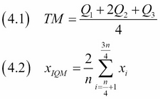
The truncated mean discards the data at given percentiles—for instance, from the lowest value to the 5th percentile and from the 95th percentile to the highest value. The trimean (4.1) is a weighted average of the median, first quartile, and third quartile. For the IQM (4.2), we discard the lowest and highest quartile of the data, so it is a special case of the truncated mean. We will calculate these measures with the SciPy tmean() and trima() functions.
We will take a look at the central tendency for varying levels of truncation with the following steps:
- The imports are as follows:
import matplotlib.pyplot as plt from scipy.stats import tmean from scipy.stats.mstats import trima import numpy as np import dautil as dl import seaborn as sns from IPython.display import HTML context = dl.nb.Context('central_tendency') - Define the following function to calculate the interquartile mean:
def iqm(a): return truncated_mean(a, 25) - Define the following function to plot distributions:
def plotdists(var, ax): displot_label = 'From {0} to {1} percentiles' cyc = dl.plotting.Cycler() for i in range(1, 9, 3): limits = dl.stats.outliers(var, method='percentiles', percentiles=(i, 100 - i)) truncated = trima(var, limits=limits).compressed() sns.distplot(truncated, ax=ax, color=cyc.color(), hist_kws={'histtype': 'stepfilled', 'alpha': 1/i, 'linewidth': cyc.lw()}, label=displot_label.format(i, 100 - i)) - Define the following function to compute the truncated mean:
def truncated_mean(a, percentile): limits = dl.stats.outliers(a, method='percentiles', percentiles=(percentile, 100 - percentile)) return tmean(a, limits=limits) - Load the data and calculate means as follows:
df = dl.data.Weather.load().resample('M').dropna() x = range(9) temp_means = [truncated_mean(df['TEMP'], i) for i in x] ws_means = [truncated_mean(df['WIND_SPEED'], i) for i in x] - Plot the means and distributions with the following code:
sp = dl.plotting.Subplotter(2, 2, context)
cp = dl.plotting.CyclePlotter(sp.ax)
cp.plot(x, temp_means, label='Truncated mean')
cp.plot(x, dl.stats.trimean(df['TEMP']) * np.ones_like(x), label='Trimean')
cp.plot(x, iqm(df['TEMP']) * np.ones_like(x), label='IQM')
sp.label(ylabel_params=dl.data.Weather.get_header('TEMP'))

cp = dl.plotting.CyclePlotter(sp.next_ax())
cp.plot(x, ws_means, label='Truncated mean')
cp.plot(x, dl.stats.trimean(df['WIND_SPEED']) * np.ones_like(x),
        label='Trimean')
cp.plot(x, iqm(df['WIND_SPEED']) * np.ones_like(x), label='IQM')
sp.label(ylabel_params=dl.data.Weather.get_header('WIND_SPEED'))

plotdists(df['TEMP'], sp.next_ax())
sp.label(xlabel_params=dl.data.Weather.get_header('TEMP'))

plotdists(df['WIND_SPEED'], sp.next_ax())
sp.label(xlabel_params=dl.data.Weather.get_header('WIND_SPEED'))
plt.tight_layout()
HTML(dl.report.HTMLBuilder().watermark())
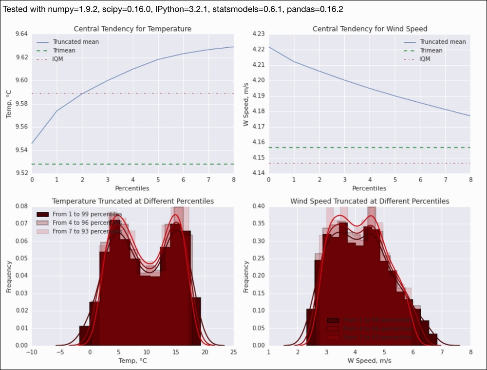
Refer to the following screenshot for the end result (refer to the central_tendency.ipynb file in this book's code bundle):
- The SciPy documentation for
trima()at https://docs.scipy.org/doc/scipy/reference/generated/scipy.stats.mstats.trima.html (retrieved August 2015) - The SciPy documentation for
tmean()at https://docs.scipy.org/doc/scipy/reference/generated/scipy.stats.tmean.html#scipy.stats.tmean (retrieved August 2015)