Most time series modeling depends on the data being stationary. The easiest definition of a stationary time series is that most of its statistical characteristics are all roughly constant over time. For statistical characteristics, the mean, variance, and autocorrelation are most commonly mentioned. For this to be true, we cannot have any trends, that is, data cannot increase monotonically over time. There cannot be long cycles of ups and downs either. If any of these things are true, the mean will change over time and the variance too. There are other more complex mathematical tests, such as the following (Augmented) Dickey-Fuller test. We focus on this test here as it is conveniently available in statsmodels.

The fact is that when doing time series analysis, we first need to make sure that the data is stationary. The easiest way to check whether your data is stationary in Python is to do an Augmented Dickey-Fuller test. This is a statistical test that estimates if your dataset is stationary. The statsmodels package has a function that tests this and sends back the diagnostics. The value of the test (we will call it the ADF value) needs to be compared to the critical values at 1, 5, and 10%. If the ADF value is below the critical value at 5% and the p-value (yes, the statistical p-value) is small, around less than 0.05, we can reject the null hypothesis that the data is not stationary at a 95% confidence level.

To make it easier to figure out if the results show whether the time series is stationary or not, let's write a small function that runs the function and summarizes the output:

def is_stationary(df, maxlag=15, autolag=None, regression='ct'): 
    """Run the Augmented Dickey-Fuller test from Statsmodels 
    and print output. 
    """ 
    outpt = stt.adfuller(df,maxlag=maxlag, autolag=autolag, 
                         regression=regression) 
    print('adf		 {0:.3f}'.format(outpt[0])) 
    print('p		 {0:.3g}'.format(outpt[1])) 
    print('crit. val.	 1%: {0:.3f},  
          5%: {1:.3f}, 10%: {2:.3f}'.format(outpt[4]["1%"],  
          outpt[4]["5%"], outpt[4]["10%"])) 
    print('stationary?	 {0}'.format(['true', 'false'] 
          [outpt[0]>outpt[4]['5%']])) 
    return outpt 

We are now ready to test the stationarity of a dataset, so let's read one in.

This dataset can be downloaded from DataMarket ( https://datamarket.com/data/set/22n4/ ). The data comes from the Time Series Data Library ( https://datamarket.com/data/list/?q=provider:tsdl ) and originated in Abraham and Ledolter (1983). It shows the monthly car sales in Quebec from 1960 to 1968. As before, we use a date parser to get a Pandas time series DataFrame directly:

carsales = pd.read_csv('data/monthly-car-sales 
                       -in-quebec-1960.csv', 
                       parse_dates=['Month'],  
                       index_col='Month',  
                       date_parser=lambda d:    
                       pd.datetime.strptime(d, '%Y-%m')) 

To go over to a Pandas Series object instead of DataFrame, we do the same thing as before:

carsales = carsales.iloc[:,0] 

Plotting the dataset shows some interesting things. The data has some strong seasonal trends, that is, cyclical patterns within each year. It also has a slow upward trend but more on that later:

plt.plot(carsales) 
despine(plt.gca()) 
plt.gcf().autofmt_xdate() 
plt.xlim('1960','1969') 
plt.xlabel('Year') 
plt.ylabel('Sales') 
plt.title('Monthly Car Sales'), 

We can now run our small wrapper to test if it is stationary:

is_stationary(carsales); 

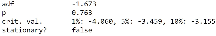
It is not! Well, this is not a huge surprise as it had all those patterns. This takes us to the next section, where we will look at various patterns and components that time series is made up of.