
In this appendix, we will cover several things that will help you when doing data analysis in Jupyter Notebook and compiling reports. This appendix covers the following topics:
- General Jupyter Notebook tips and tricks:
- Useful keyboard shortcuts to speed up your workflow
- A short introduction to the Markdown syntax to edit text cells
- A few other useful tips
- Jupyter Notebook extensions
- Matplotlib styles for pretty plotting from the start
- Useful resources such as data repositories, Python packages, and similar
The various tips and tricks are not crucial for data analysis in Python, but it is very useful to make the workflow better and easier to pick up right where you left off in a project. Let's jump right in and start off by looking closer at some good things about Jupyter Notebook.
Jupyter Notebook is an interactive web application that sends/receives data from a programming language kernel. In this book, we have worked in Python; it is also possible to work in several other programming languages in Jupyter Notebook. The notebook format has support for what it calls checkpoints—when you save, it will create a checkpoint and you can always roll back to that previous checkpoint from File |Revert to Checkpoint in the menu.
One of the most important problems that Jupyter Notebook solves is that it provides a full record of your data analysis session; this record along with the data files is all that anyone needs to reproduce your analysis. The record may contain, except the code, (structured) text, images, videos, equations, and even interactive widgets. The notebook can be compiled into other formats that are easier to share, such as PDF and HTML. In addition to these things, it is possible to extend the functionality of Jupyter Notebook with extensions. After looking at some of the more useful keyboard shortcuts, we will go through a few of these extensions.
First, I would like to go through a few of the most useful keyboard shortcuts. The general approach to keyboard shortcuts in Jupyter Notebook is very simple. It has two main modes: command and edit mode. As you might have suspected, edit mode is when you edit text in a cell and command mode is when you run commands in your notebook. The available keyboard shortcuts are of course reflected in what mode you are in. However, in both modes, Shift + Enter will run the current cell and Ctrl + S will save the notebook (and create a checkpoint).
Once in command mode, either by pressing Ctrl + M or Esc , the following keyboard shortcuts are available:
- B/A : This creates a new cell, B below or A above the current cell.
- X/C/V : This cuts, copies, and pastes the cell, just like you are used to in other programs. Pasting the cell here will paste it below the current cell.
- D, D : This deletes a cell.
- Z : This undoes the deletion.
- L : This shows line numbers. This is especially useful when getting error messages with a reference to a line number in your code where it breaks.
- M : This converts the current cell to a Markdown cell.
- Shift + M : This merges the current cell with the cell below.
- O : This toggles to show/hide the output shown directly below the cell.
- H : This shows all the keyboard shortcuts.
- Enter : This enters edit mode of the selected cell.
When you are in edit mode, by pressing Enter while selecting the cell you want to edit, you can do the following actions:
- Tab : Indent, or tab completion; that is, start typing a command, tab will list available commands/methods/objects/variables to complete with that are present in the name space.
- Ctrl + Shift + - : This splits a cell at the current line
- Ctrl + A : This selects all content in a cell
- Ctrl + Z : This is for undo
- Ctrl + Shift + Z : This is for redo
- Esc : This enters command mode
As mentioned, these are some of the keyboard shortcuts available. These are the ones that are the most useful in my opinion. If you want to look at all of them, enter command mode and press H .
In a Markdown cell that is created by selecting an existing cell and pressing M , you can perform the following functions:
- Create headings by preceding the text by a hash and space, "
#". - Type normal text, just like in any text editor. You can style the text as follows:
- Italics by surrounding the text with stars, that is, *text*
- Bold by surrounding the text with two stars, that is, **text**
- Make bullet lists by preceding each bullet item with a star, as follows:
* Item1 * Item 2 * Sub-item1 - Include a URL by typing
[your link text](http://your-url.com). - Include an image with
. - Make a numbered list by preceding each item in the list with a number.
If you convert a cell to Markdown text, but want to convert it back to a code cell, you simply press Ctrl + M or Esc to enter command mode and then Yto convert the selected cell.
Markdown syntax is very extensive and Jupyter Notebook follows much of the same syntax as that used at GitHub; thus, for more information on what can be done, see https://help.github.com/articles/basic-writing-and-formatting-syntax/ . Some of the possibilities are also shown in the accompanying notebook of this appendix.
Jupyter's functionality can be extended with extensions. Some of the extensions rely only on Jupyter, while others rely on external libraries and software. A few of them are inspired by plugins or functions of the CodeMirror online JavaScript editor ( https://codemirror.net ). A collection of Python-specific extensions can be installed from the IPython-contrib repository on GitHub. The URL for the collection is https://github.com/ipython-contrib/IPython-notebook-extensions . In this appendix, we will cover some of these extensions.
To install the collection of extensions along with the extension manager from the Anaconda repository, follow these steps:
- Start an Anaconda command prompt and run the following:
conda install -c https://conda.binstar.org/juhasch nbextensions - To activate some of the extensions that we want to use, start Jupyter Notebook.
- Open a new browser tab and go to
http://localhost:8888/nbextensions(where8888is the port that Jupyter listens to). - The page that you are presented with should look something like the following screenshot. The page is basically a list of the available extensions with checkboxes to activate them. If you click on the name of an extension, the page will load details about that extension:
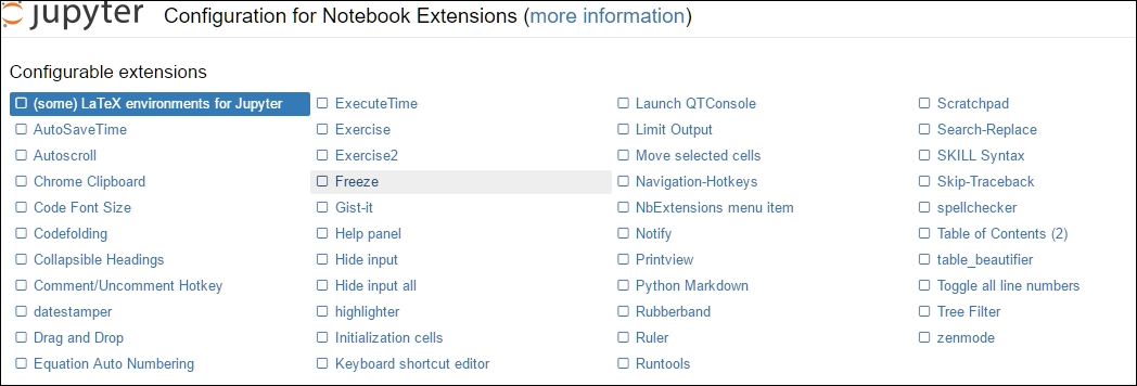
- Now, by clicking on the checkbox next to the names, activate the following extensions that we will go through (alphabetical order):
- Codefolding
- Collapsible Headings
- Help panel
- Initialization cells
- NbExtensions menu item
- Ruler
- Skip-Traceback
- Table of Contents (2)
When you have done these things, each extension will have the checkbox next to it marked, as shown in the following screenshot:

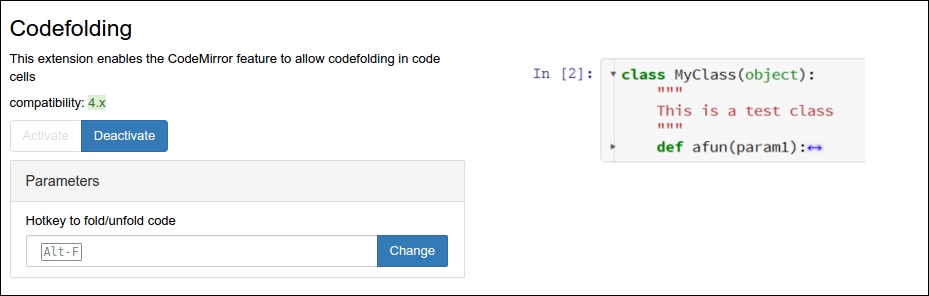
In my experience, the click response is a bit buggy, so make sure that they are all marked. After selecting all the specified extensions to be activated, you can also configure some of them. We will look at each of them separately, but the general layout revealed by clicking on the name of each extension is as follows:
- The name of the extension
- A short description
- Which versions of Jupyter Notebook it is compatible with
- An activation/deactivation button
- An image to the right, showing roughly what it does
- Possible parameters/settings for the extension
After this, the interface will grab and output the readme file, which is in Markdown syntax. In this file, the author of the extension puts any additional information that might be useful. In the coming sections, we will go through the extensions one by one.
The codefolding extension is a simple yet very useful extension. It will fold the indented lines of code, for example, functions or classes can be folded. Furthermore, it will also give you the option of folding at comments. The top of the information pane for this extension is shown here:
As an example of what you see in the readme file, I'll show you the top of the codefolding extension readme that Jupyter Notebook outputs here:
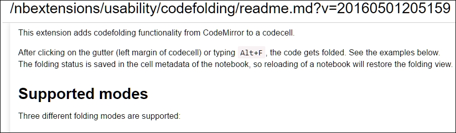
The readme is simply a more extensive description with figures and external links. With the codefolding extension, it is possible to hide long code snippets and functions within a cell. This is shown in the following example. The first image shows an arbitrary function in the way it looks in Jupyter Notebook:
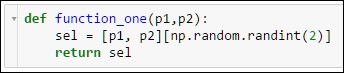
Clicking on the small arrow in the left margin will collapse the code into one line. It will then look like this:
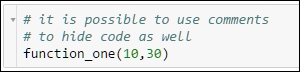
As you can see in the first image of this section showing the parameters for this extension, the keyboard shortcut Alt + F will toggle the folding. Folding will also work on nested functions and statements; for each indentation level, you can fold the code. You can collapse code cells with comments as the first line as well:
Once again by clicking on the arrow, you will collapse the rest of the code in the whole cell below it:
This is a very useful extension when you tend to write long functions or code, perhaps a plot with many different components, or if you have help functions written in the notebook.
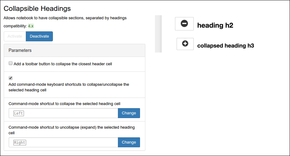
With the collapsible heading extension, it is possible to group whole sections of cells by creating Markdown cells and defining headings. Normally, this would only display the text as a heading. The extension makes the heading and all cells below it collapsible—it will collapse everything below it until a heading of equal or greater level is encountered. The available parameters in the settings page are shown here:
You can set the keyboard shortcuts to (un)collapse a selected heading, add a toolbar button, and toggle the use of keyboard shortcuts. An example of what the results of using the extension are shown here:
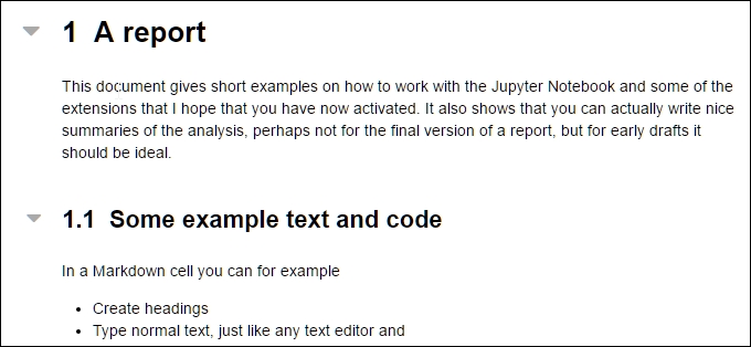
Clicking on the little arrow to the left of the heading will collapse the heading and everything below it under the same section. It will then look like the following image:

This is very helpful when you are doing multiple analyses of similar or the same data. Try opening up one of the chapters that we worked on in the book with the extension active, and you will see the usefulness of this.
The help panel is useful when you start out writing your own code in Jupyter Notebook, as it has the possibility of displaying all the keyboard shortcuts in a panel alongside your notebook. The top of the details page for the extension looks as follows:
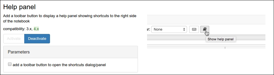
Here, you can check the box for add a toolbar button to open the shortcuts dialog/panel . Then you will have a button, as is shown to the right in the preceding image.
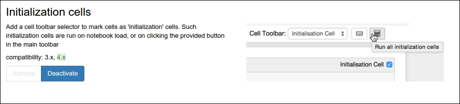
Much of the code in the beginning of an analysis session is something that you want to run every time it is opened. The initialization cells extension alleviates this by adding two things—a cell toolbar that allows you to mark initialization cells and a button to rerun all these marked initialization cells. The following image shows the details page of the extension, and to the right is the button to trigger the rerunning of the initialization cells:
To use this extension, perform the following steps:
- When activated, go and open a notebook and create the cells you want to have for starters. The accompanying example notebook has some initialization cells in it.
- To change cells into initialization cells, you navigate to View | Cell Toolbar | Initialization Cell. When you have clicked this, each cell will get a toolbar (that is, cell toolbar) with a checkbox in the upper right corner, as shown in the following image:
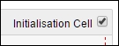
- Click on the checkbox for the cells that you want to run automatically when you open the notebook, for example, cells with imports, data reading, and data cleaning.
- Now, close the notebook, open it again, and watch the checked cells run automatically. You can also trigger this by clicking on the button that looks like a calculator; see the first image of this section.
This extension is very useful because sometimes we have to restart our kernel or notebook and when this happens, it is not that much fun to have to rerun all the cells that simply import modules and load data.
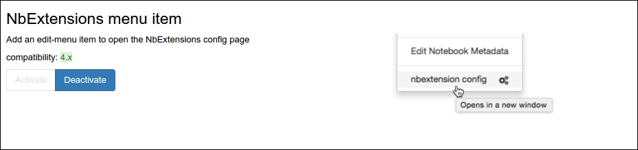
The NbExtensions menu item extension is very simple; it adds a menu item to open the extensions settings page where you can activate/deactivate extensions. The menu item can be found under the Edit item. The following is a screenshot from the extension details page showing the menu item to the left:
The ruler is a simple extension and is for aesthetics so that you know when to wrap your code for it to follow standards. The available parameters are the column width and the color of the ruler and its line style, as shown in the following image:
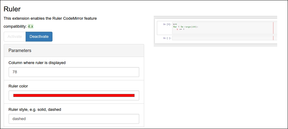
The extension will draw a vertical line in each cell at the column width given in the parameters. The following image shows what it looks like:
Sometimes there is an exception raised in the code that you run in a cell. When the stack trace to the exception is long, Jupyter Notebook will still display the whole trace. It can be a bit tedious to scroll to the bottom of the cell output to get to what caused the exception. There are no parameters to set for this extension. To give you a good example of this, I found a filed bug in the current version of NumPy giving a long trace. You can read about the bug at https://github.com/numpy/numpy/issues/7547 . To test the skip-traceback extension, follow these instructions:
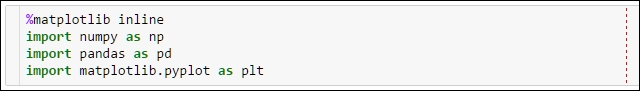
- After the standard imports (with the extension activated as we described before), run the following:
values = (1+np.array([0, 1.e-15]))*1.e27 plt.plot(values) - You should now see something like the following screenshot:
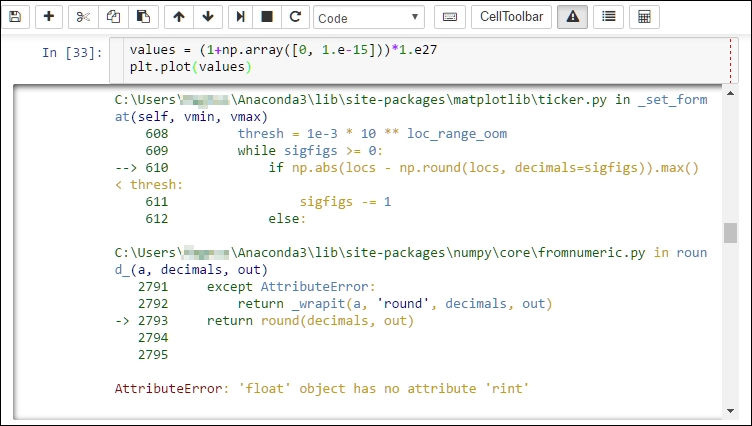
- The trace is really long; you have to scroll through a long list of pointers and files. Now, click on the button on the toolbar that shows a triangle and an exclamation mark (see the preceding and following images); it toggles the hiding of the traceback.
- Run the code again and you get the following:
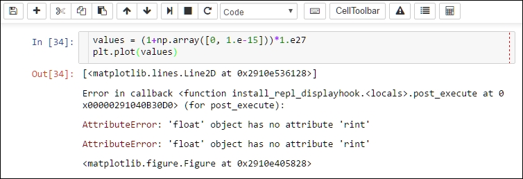
This is much better and less confusing and shows why skipping traceback is very useful sometimes. There are of course situations when viewing the full trace is useful, for example, when you want to report a bug.
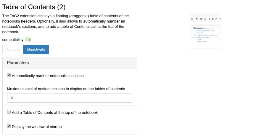
The collapsible headings extension is good when working with long notebooks with multiple sections. The table of contents is useful when navigating around in such notebooks. The plugin only has a few parameters. You can let it number sections, choose to what depth the table of contents go to, and toggle if it should show a floating window or a table at the top of the notebook. Some of these can be set in the floating window as well:
In the notebook, you can toggle the floating window with the table of contents by pressing the button. This is shown in the following image:

Once you have pressed the button, the floating window will appear to the right. For the example notebook of this appendix, it will look like the following:
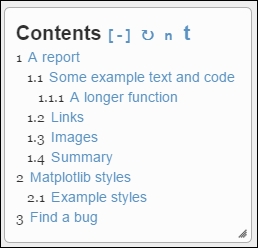
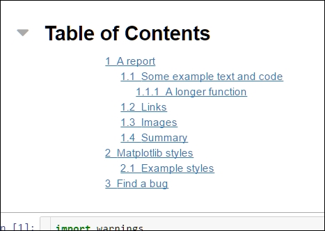
Here, you have four buttons next to Contents, except for the clickable headings of the table. Clicking on the headings will take you to that part of the notebook. The first button, [-], will simply collapse the table of contents, and the button next to it will reload it; n will toggle the section numbering in the notebook; lastly, the t will toggle a table of contents at the top of the notebook in a separate cell. The output of clicking on the last button is shown here:
Here, I will give you some extra tips on using Jupyter Notebook. There are many things you can use it for and that is what makes it so good.
Starting Jupyter Notebook with the extra flag -ip *, or an actual IP instead of *, will allow external connections, that is, on the same network as your computer (or the Internet if you are connected directly). It will allow others to edit the notebook and actually run code on your computer, so be very careful with this. The full call would look as follows:
jupyter notebook -ip *
It can be useful in educational settings where you want people to be able to focus on coding and not installing things or if they do not have the right version of a certain package.
All the notebooks can be exported to PDF, HTML, and other formats. To reach this, navigate to File | Download as in the menu. If you export in PDF, then you might want to put the following in a cell at the beginning of your notebook. It will try to make PDF versions of your figures first, which will be vector-based graphics and thus lossless when you resize them and eventually be of better quality when incorporated into the PDF:
ip = get_ipython()
ibe = ip.configurables[-1]
ibe.figure_formats = { 'pdf', 'png'}
print(ibe.figure_formats)
To export to PDF, you need other external software—a Latex distribution ( https://www.latex-project.org ) and Pandoc ( http://pandoc.org ). Once installed, you should be able to export your notebook to PDF; any Latex compilation errors should show up in the terminal that you started Jupyter Notebook from.
It is also possible to edit any other text file with Jupyter. In the Jupyter dashboard, that is, the main page that is opened when you start it, you can create new files that are not notebooks:
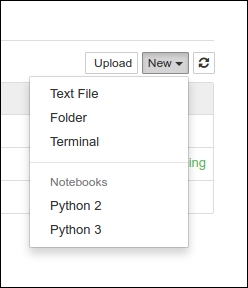
To give you an idea, I have included additional files in the appendix data files—one text file in Markdown format (ending with .md) and a file called helpfunctions.py with the despine() function that we created in previous chapters. In addition to these two, you also have the mystyle.mplstyle file to edit. In the editor, you can choose what format the file is in, and you will get highlighting for it.