
In this example, we will look at a cluster finding algorithm in Scikit-learn called DBSCAN. DBSCAN stands for Density-Based Spatial Clustering of Applications with Noise, and is a clustering algorithm that favors groups of points and can identify points outside any of these groups (clusters) as noise (outliers). As with the linear machine learning methods, Scikit-learn makes it very easy to work with it. We first read in the data from
Chapter 5
, Clustering, with Pandas' read_pickle function:
TABLE_FILE = 'data/test.pick'
mycat = pd.read_pickle(TABLE_FILE)
As with the previous dataset, to refresh your memory, we plot the data. It contains a slice of the mapped nearby Universe, that is, galaxies with determined positions (direction and distance from us). As before, we scale the color with the Z-magnitude, as found in the data table:
fig,ax = plt.subplots(1,2, figsize=(10,2.5))
plt.subplot(121)
plt.scatter(mycat['Y'], -1*mycat['X'],
            s=8,
            color=plt.cm.viridis_r(
                    10**(mycat.Zmag-mycat.Zmag.max()) ),
            edgecolor='None')
plt.xlabel('Y (Mpc)'), plt.ylabel('X (Mpc)')
ax = plt.gca()
despine(ax)
ax.locator_params(axis='x', nbins=5)
ax.locator_params(axis='y', nbins=5)
plt.axis('equal')
plt.subplot(122)
c_arr = 10**(mycat.Zmag-mycat.Zmag.max())
plt.scatter(-1*mycat['X'],mycat['Z'],
            s=8,
            color=plt.cm.viridis_r(c_arr),
            edgecolor='None')
lstyle = dict(lw=1.5, color='k', dashes=(6,4))
ax = plt.gca()
despine(ax)
ax.locator_params(axis='x', nbins=5)
ax.locator_params(axis='y', nbins=5)
plt.plot([0,150], [0,80], **lstyle)
plt.plot([0,150], [0,45], **lstyle)
plt.plot([0,-25], [0,80], **lstyle)
plt.plot([0,-25], [0,45], **lstyle)
plt.xlabel('X (Mpc)'), plt.ylabel('Z (Mpc)')
plt.subplots_adjust(wspace=0.3)
plt.axis('equal'),
plt.ylim((-10,110));
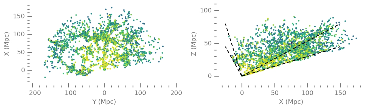
The data spans extremely large scales and many galaxies in the given directions. To start using machine learning for cluster finding, we import the relevant objects from Scikit-learn:
from sklearn.cluster import DBSCAN
from sklearn import metrics
from sklearn.preprocessing import StandardScaler
The first import is simply the DBSCAN method, and the second import is the metrics module with which we can calculate various statistics on the clustering algorithm. The StandardScaler class is simply to scale the data, as in
Chapter 5
, Clustering. Next, we set up the input data; every row should contain the coordinates of a feature/point scaled. This scaled coordinate list is then input into the DBSCAN method:
A = np.array([mycat['Y'], -1*mycat['X'], mycat['Z']]).T
A_scaled = StandardScaler().fit_transform(A)
dbout = DBSCAN(eps=0.15, min_samples=5).fit(A_scaled)
The DBSCAN object is instantiated with several parameters. The eps parameter limits the size of the cluster in terms of the distance within which at least min_samples have to lie for it to be a cluster (remember, in scaled units). The dbout object now stores all the results of the fit. The dbout.labels_ array contains all the labels for each point; points not in any cluster are given a -1 label. Let's check whether we have any:
(dbout.labels_==-1).any()
It prints out True, so we have noise. Another important method that the output object has is core_sample_indices_. It contains the core samples from which each cluster is expanded and formed. It is almost like the centroid positions in k-means clustering. We now create a Boolean array for the core sample indices and also a list of the unique labels in the results. This is the recommended way according to the Scikit-learn documentation.
csmask = np.zeros_like(dbout.labels_, dtype=bool)
csmask[dbout.core_sample_indices_] = True
unique_labels = set(dbout.labels_)
Without the true labels of the clusters, it is tricky to measure the success of the cluster finding. Normally, you would calculate the silhouette score, which is a score that scales with the distance between the centroid and samples in the same cluster and nearby clusters. The higher the silhouette score, the better the cluster finding was at defining the cluster. However, this assumes clusters that are centered around one point, not a filamentary structure. To show you how to calculate and interpret the silhouette score, we go through it for this example, but keep in mind that it might not be a representative method in this case. We will calculate the silhouette score and also print out the number of clusters found. Remember that the labels array also contains the noise labels (that is, -1):
n_clusters = len(set(labels)) - [0,1][-1 in labels]
print('Estimated number of clusters: %d' % n_clusters)
print("Silhouette Coefficient: %0.3f"
      % metrics.silhouette_score(A_scaled, dbout.labels_))
Silhouette score values close to zero indicate that the clusters overlap. Now we will plot all the results and check what it looks like. I have tried to plot the core samples differently by increasing their marker size and decreasing the size of non-core samples. I also shuffled the colors in an attempt at making different clusters stand out against their neighbors:
colors = plt.cm.viridis(np.linspace(0.3, 1, len(unique_labels)))
np.random.seed(0)
np.random.shuffle(colors)
for lbl, col in zip(unique_labels, colors):
    if lbl == -1:
        # Black used for noise.
        col = 'DarkRed'; m1=m2= '+'; s = 10; a = 0.5
    else:
        m1='.';m2='.'; s=5; a=1
    cmmask = (dbout.labels_ == lbl)
    xy = A[cmmask & csmask]
    plt.scatter(xy[:, 0], xy[:, 1], color=col,
                marker=m1,
                s=s+1,
               alpha=a)
    xy = A[cmmask & ~csmask]
    plt.scatter(xy[:, 0], xy[:, 1], color=col,
                marker=m2,
                s=s-2,
               alpha=a)
despine(plt.gca())
noiseArtist = plt.Line2D((0,1),(0,0),
                       color='DarkRed',
                       marker='+',
                       linestyle='',
                       ms=4, mew=1,
                       alpha=0.7)
clusterArtist = plt.Line2D((0,1),(0,0),
                       color='k',
                       marker='.',
                       linestyle='',
                      ms=4, mew=1)
plt.legend([noiseArtist, clusterArtist],
           ['Outliers','Clusters'],
           numpoints=1)
plt.title('A slice of the Universe')
plt.xlabel('X [Mpc]')
plt.ylabel('Y [Mpc]'),
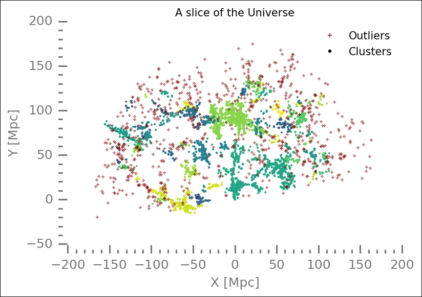
The algorithm also finds noise (outliers), which are plotted in red crosses here. Try to tweak the displaying of the core and non-core samples so that they stand out more. Furthermore, you should try different parameters for the DBSCAN method and see how the outcome is affected. Another thing would be to go back to Chapter 5 , Clustering, and put 66 clusters in the hierarchical cluster algorithm that we tried there with the same dataset and compare.