3.6 Discriminant Saliency Based on Centre–Surround

Discriminant analysis is a technique that has frequently been applied in pattern recognition. Its objective is to classify a set of observed data into predefined classes such that the expected error probability tends to be minimum. Discriminant analysis needs to build a discriminant function or criterion based on a set of observed data in which the classes are known (as the training set), and the discriminant function or criterion is used to predict the class of new observed data with unknown class. Sometimes this discriminant function is implemented to select features of recognized objects, determining which features can distinguish one class from all others. Since these observed data are often uncertain, the method is rooted in statistical signal processes such as signal detection and estimation mentioned in Section 2.6, with decision theory and information theory. Decision theory is to select or find the optimal decision scheme by a quantitative method according to the information criterion. A discriminant saliency (DISC) model is based on decision theory.

The first literature on DISC modelling is proposed by Gao et al. [39]. It is formulated as a recognition problem, that is to recognize the classes of some objects in a scene by selecting optimal features that most discriminate one class from the others. Optimal feature selection is just like saliency determination in the given object context. For instance, the shape and contour features indicate the saliency for a green car against its surroundings of green trees, and also distinguish the green car from green trees; and the colour feature will indicate saliency and also recognize a red apple among green capsicums; therefore, the two concepts of saliency detection and object discrimination/recognition with feature sets are equated [39]. In the meantime, a hypothesis was proposed that all saliency decisions are optimal in the theoretic sense of a decision [39]. The discriminant criterion of feature selection in [39] is implemented by maximization of mutual information between features and class labels. Due to the dependence of this model on a given object, it is considered to be top-down discriminant saliency detection. However, the idea of DISC can easily be extended to bottom-up saliency computation by the local centre–surround process [8, 40, 41], and this will be the main topic to be discussed in this section.

The term ‘centre–surround’ is familiar to readers since it has already been mentioned several times in this book. In the retina of our visual system, the receptive field of the ganglion cells has a centre–surrounding opponent structure (Section 2.1.3). It can be described as the difference between two Gaussian functions (Equation 2.3). In the BS model, the centre–surround is evaluated by using difference with different scales in an image pyramid (Section 3.1). In the AIM model, self-information of an image patch is based on its surrounding image patches. The DISC model of pure bottom-up saliency is to calculate the discriminant power of a set of features related to the binary-classification problem based upon the opposed stimuli at a centre and its surround. The discriminant criterion is maximization of mutual information across all features; for example Class 1 denotes the centre window and Class 0 is the surround window at each location of an input image. In the following, we will introduce the discriminant criterion, probability density estimation, computational parsimony of discriminant criterion and model implementation.

3.6.1 Discriminant Criterion Defined on Centre–Surround

As already mentioned, the centre–surround process in early vision is important for determining the saliency of each location in a scene, and is generally considered within most of computational models. It is known that the larger the difference of stimuli located at the centre and its surrounding is, the more salient the location becomes. The centre–surround process in the DISC model is from an alternate view that combines the hypothesis of decision for theoretic optimality [8]. Without high-level information which is available in conventional discriminant analysis (i.e., knowing class labels in the training set), binary class labels are defined: Label 1 for the centre area and Label 0 for its surround. Then the two classes are computed on a set of pre-extracted features.

Without loss of generality, let us consider the saliency measurement of a location region with its neighbouring region on an input image. Let denote a centre window and denote a surround window of location l, where the superscript {0,1} denotes the class labels and the subscript l is the location index under consideration.

The feature responses in the two windows are observed from a random process with k dimensions , where k represents the number of features that can discriminate between the centre and the surround windows at region location l, and is the class label, where , c = 1 for the centre window and c = 0 for the surround window . The feature vector observed from location (i, j) within the two windows ( and ) is represented as , where and the feature vectors in all possible locations (i, j) in both window, related to location l, are independently drawn from the label-conditional probability densities , so feature vector x can be regarded as a random vector extracted from the region related location l and its label c also is a random variable. In order to measure the discrimination of the feature vector for the two labels in a region related to location l, mutual information between label and feature vector is adopted in the model.

(3.41)

where denotes the mutual information and the subscript l means the mutual information only for the region related to l, is the joint probability density of the random feature vector x and random variable label c, and are probability densities for feature vector x and label c, respectively. The mutual information is to integrate all x drawn within the region related to location l for both label classes. It is obvious that when the feature vector x cannot discriminate the centre and surround windows, this means that the feature vector is independent of label c, and then the joint probability density is satisfied:

(3.42)

In this case the mutual information (Equation 3.41) equals zero. Contrarily, if the feature vector x can discriminate the centre and surround windows – that is feature vector x and the label c are more correlative – the mutual information has a larger value. Thus, the mutual information of the local region just represents the saliency of the location l, and we have

(3.43)

If the number of features is one (i.e., k = 1) and the class label is equiprobable, Equation 3.41 can be regarded as the summation of two KL divergences defined at the centre and surround windows between the conditional probability density and the whole probability density of the feature at location l. Equation 3.41 can therefore be rewritten as

(3.44)

where the conditional probability density is given by

and the KL divergence is given by

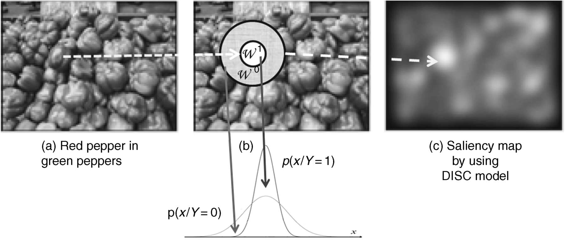
KL divergence was mentioned in Section 2.6.2 (Equation 2.9). It can be seen from Equation 3.44 that a higher salient location means that the difference of probability density between the centre and surround including the centre windows is larger. A sample for the probability densities of the centre window and the whole window related to location l is shown in Figure 3.14, which only considers the case with one colour feature (k = 1). When k > 1, the joint density covering all features in both windows should be computed, and this is very complex. Apparently, the key issue to calculate the local saliency from Equation 3.43 is firstly to estimate the local probability density.

Figure 3.14 Illustration of the discriminant centre–surround saliency for one feature (a) original image; (b) centre and surround windows and their conditional probability density distribution; (c) saliency map colour feature (k = 1).

3.6.2 Mutual Information Estimation

In the DISC model, the mutual information estimation in each location of an image is based upon two strategies for approximation: (1) the whole mutual information for a high dimension feature vector in Equation 3.41 can be replaced by the sum of marginal mutual information between every individual feature and its class label; (2) each marginal density is approximated by a generalized Gaussian function.

The reason why these are tenable is a statistical property of band-pass natural image features: all features in the window under consideration are obtained by band-pass filters (such as wavelet or Gabor) [8, 40]. Therefore, as we shall show, mutual information estimation is based on wavelet coefficients (Gabor filter can be regarded as one kind of wavelet filters).

1. Marginal mutual information and saliency map

The wavelet transform of a natural image decomposes the image into several component images at different scales from coarse resolutions to fine resolutions (i.e., parent, children, grandchildren and so on) at three orientations by different band-pass filters. In some literature, it has been observed that for different kinds of images the conditional probability density of the co-location wavelet coefficients for its parent is invariable, or there is a statistical dependence between an arbitrary coefficient and its parent [41–44]. For instance, the probability density of arbitrary wavelet coefficients for its parent scale appears the same bow-tie shape [41, 42]. This statistical dependence carries little information about image class. If these wavelet coefficients are considered as the features of the DISC model, the property of statistical dependence can be used to reduce the computational complexity of calculating the saliency map, because the dependence between features is the same, no matter which class (i.e., the centre or surround window) is in a considered location. Mathematically, feature dependence is described as mutual information between features. For a given feature x_d of both centre and surround windows at location l, the mutual information between the dth feature and its previous (d − 1) feature is expressed as

Consider the property of statistical dependence covers all k features, we have

(3.45)

where class label Y {0, 1}. Equation 3.45 can be used to simplify the computation of Equation 3.41 by the marginal mutual information according to the following theorem proved in [41].

Theorem 3.1 [41] Let be a collection of features and Y be the class label. If

According to Theorem 3.1, the saliency map at location l, considering Equations 3.41 and 3.43, can be rewritten as

(3.46)

where is the marginal mutual information of feature , at location l.

2. Estimation of marginal mutual information

From the definition of one-dimensional mutual information, the calculation of needs to estimate two probability densities: one is the marginal density of feature , and the other is its conditional density, conditioned on its class Y. Fortunately, this is not difficult because it has already been confirmed that these probability densities for band-pass features in natural images can be well approximated by generalized Gaussian distributions (GGDs) [45–47]. Its form is

(3.47)

where

being a gamma function, and α and β are the parameters for scale and shape, respectively. The parameter β controls the attenuation rate from the peak value, which forms different families of GGDs. When β = 2, Equation 3.47 is Gaussian family and when β = 1, it is Laplacian family. In [42, 46, 48], it has been observed that wavelet sub-band coefficients have highly non-Gaussian statistics, because the histograms for coefficients are more sharply peaked at zero with more extensive tails. Experimental comparisons [42, 46, 48] showed that the probability density function of wavelet coefficients is closer to a Laplacian distribution, that is β ≈ 1. The marginal mutual information for one feature by making use of Equation 3.47 has the following form [40]:

(3.48)

The conditional probability density and the probability density of feature x_d are presented as GGD with different parameters, so the KL divergence in Equation 3.48 can be written as

where, α₁, β₁, α₂ and β₂ are the parameters for the two GGDs, respectively.

The estimation of parameters α and β is via the following moment equations [40, 42, 43, 45].

(3.49)

where symbols σ and κ are the two-order and four-order moments of feature x, variance and kurtosis, which can be estimated by

(3.50)

where E_x denotes the expectation of feature x. Apparently, parameter estimation (Equation 3.49 only requires sampling the feature responses within the centre window or the surround window, and then the KL divergence in Equation 3.48 is easily estimated. For simplicity, we set β = 1, and then α only depends on the variance. The GGD parameters of a feature's probability density in the centre, surround and total (centre + surround) windows can be quickly obtained.

In summary, the well-known statistical property in band-pass features enables the computation of high dimensional probability density to be replaced by a number of marginal densities of each feature, and the KL divergence of each feature is estimated by the GGD parameters. Consequently, the estimation for the total mutual information is the sum of the marginal mutual information of all features at each location. According to Equation 3.46, the salient value in each location can be computed, and then the final saliency map is obtained.

3.6.3 Algorithm and Block Diagram of Bottom-up DISC Model

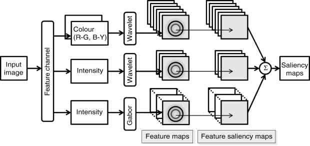
For an input image I, the algorithm of the bottom-up DISC model mainly has four stages, as follows.

Figure 3.15 Block diagram of the bottom-up DISC model

The block diagram of the bottom-up DISC model is shown as Figure 3.15.

It is worth noting that the choice of feature sets is not crucial in the DISC model. Different types of wavelet filters can be used. The DISC model is rooted in decision theory of statistical signal processing that has previously been used in top-down object detection and recognition. The idea is extended to bottom-up saliency which is based on the following hypothesis: The most salient locations in the visual filed are those that can distinguish between the feature responses in the centre and its surround with the smallest expected probability of error [40]. Therefore it can be easy to combine both bottom-up saliency and top-down saliency in a computational model and can accurately detect saliency in a wide range of visual content, from static scene to motion-occurring dynamic scene when motion feature channel is added in DISC as a feature channel [8, 40]. The comparison of the DISC model with other models (e.g., the BS model or the AIM model) shows its superiority for more criteria that are to be discussed in Chapter 6. Similar to these other computational models, the DISC model is programmable and has been coded in MATLAB® [49], so it is the choice for visual saliency computation in real engineering applications.