
8.1 Attention-modulated Just Noticeable Difference
As introduced in Chapters 1 and 2, visual attention is one of the most important mechanisms of the HVS. However, other characteristics of the HVS have also been revealed by physiologists and psychologists. One such characteristic is visual masking, and it is reflected by the concept of just noticeable difference (JND) in image processing. The JND captures the visibility threshold (due to masking) below which the change cannot be detected by the majority of viewers (e.g., 75% of them).
Visual attention and JND are different: an object with high attention value does not necessarily mean that it should have a high or low JND value, since either case is possible. If the object is attended, the visibility threshold is lower than that for the case when the object is out of focus. Visual attention and JND are both related to the overall visibility threshold. Therefore, visual attention and JND are considered simultaneously in many image processing applications to provide a more complete visibility model of the HVS, and we refer it as attention-modulated JND, or as the overall visibility threshold.
JND modelling is first briefly introduced, and then two techniques – non-linear mapping and foveation – are presented to combine visual attention with JND modelling.
8.1.1 JND Modelling
Many factors affect the JND, to account for spatiotemporal contrast sensitivity function (CSF) [1], contrast masking [2], pattern masking (including orientation masking) [3], temporal masking [4], eye movement effect [5] and luminance adaptation [6]. Although JND is difficult to compute accurately, most models create a profile (usually of the same size as the image itself) of the relative sensitivity across an image or a frame of video. Further, JND can be computed in different domains, including the sub-band and pixel domains. Two images cannot be visually distinguished if the difference in each image pixel (for pixel domain JND) or image sub-bands (for sub-band JND) is within the JND value. A sub-band-based JND model can incorporate the frequency-based HVS aspects (e.g., CSF). However, computing a pixel-based JND may be useful when a sub-band decomposition is either not available (e.g., in motion estimation [7]) or is too expensive to perform (as in quality evaluation [8]). In [9], a review of JND modelling including concepts, sub-band domain modelling, pixel domain modelling, conversion between domains, model evaluation and so on can be found. In the pixel domain, JND usually accounts for factors of spatial luminance adaptation, spatial contrast masking and temporal masking.
8.1.1.1 Spatial JND Modelling
Luminance adaptation and contrast masking are spatial masking factors. Luminance adaptation (LA) refers to the masking effect of the HVS towards background luminance. For digital images, the curve of the LA is U-shape [10–12]. A higher visibility threshold occurs in either very dark or very bright regions in an image, and a lower one occurs in regions with medium brightness. Viewing experiments have been done [11] in order to determine the relationship between the threshold and the grey level of a digital image displayed on a monitor, and the result is modelled as follows [11]:
(8.1) ![]()
(8.2) 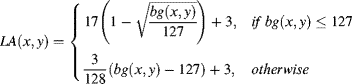
where f(.) represents the input image/frame; (![]() ) represents the image pixel position; bg is calculated as the average background luminance calculated by a 5 × 5 weighted low-pass filter B; and LA denotes the luminance adaptation.
) represents the image pixel position; bg is calculated as the average background luminance calculated by a 5 × 5 weighted low-pass filter B; and LA denotes the luminance adaptation.
Contrast masking (CM) is an important phenomenon in HVS perception and is referred to as the reduction in the visibility of one visual component in the presence of another [8]. Usually noise becomes less visible in the regions with high spatial variation, and more visible in smooth areas. CM is calculated as follows in [11]:
(8.3) ![]()
where mg(x, y) is the maximum gradient derived by calculating the average luminance changes around the pixel (x, y) in four directions as
(8.4) ![]()
(8.5) ![]()
The operators Gk are defined in Figure 8.1. The quantities ![]() and
and ![]() depend on the background luminance bg(x, y) and specify the relationship between the visibility threshold and the luminance contrast around the point (x, y), hence modelling the spatial masking.
depend on the background luminance bg(x, y) and specify the relationship between the visibility threshold and the luminance contrast around the point (x, y), hence modelling the spatial masking.
Figure 8.1 Matrix ![]() : (a)
: (a) ![]() ; (b)
; (b) ![]() ; (c)
; (c) ![]() ; (d)
; (d) ![]()

To integrate LA and CM for spatial JND (SJND) estimation, we adopt the non-linear additivity model for masking (NAMM) [14] method, which can be described mathematically as
where ![]() is the gain reduction factor to address the overlapping between two masking factors, and is set as 0.3 in [14].
is the gain reduction factor to address the overlapping between two masking factors, and is set as 0.3 in [14].
8.1.1.2 Spatial-temporal JND Modelling
In addition to the spatial masking effect, the temporal masking effect should also be considered to build the spatial-temporal JND (STJND) model for video signals. Usually, larger inter-frame luminance difference results in a larger temporal masking effect. To measure the temporal JND function, experiments on a video sequence at 30 frames/s have been constructed in which a square moves horizontally over a background. Noise has been randomly added or subtracted to each pixel in small regions as defined in [13]; the distortion visibility thresholds have been determined as a function of the inter-frame luminance difference. Based on the results, STJND is mathematically described as
(8.8) ![]()
where TJND(.) is the experimentally derived function to reflect the increase in masking effect with the increase in inter-frame changes, as denoted in Figure 8.2; and ![]() represents the average inter-frame luminance difference between the current frame t and the previous frame t − 1.
represents the average inter-frame luminance difference between the current frame t and the previous frame t − 1.
Figure 8.2 Temporal effect defined as a function of inter-frame luminance difference [13]. © 1996 IEEE. Reprinted, with permission, from C. Chou, C. Chen, ‘A perceptually optimized 3-D sub-band codec for video communication over wireless channels’, IEEE Transactions on Circuits and Systems for Video Technology, April 1996

The STJND model provides the visibility threshold of each pixel of an image by assuming that the pixel is projected on the fovea and is perceived at the highest visual acuity. However, if the pixel is not projected on the fovea, the visual acuity becomes lower. The STJND model can only provide a local visibility threshold. To measure the global visibility threshold of the whole image, the visibility threshold of the pixel not only depends on the local JND threshold, which is modelled by the STJND model, but also depends on its distance from the nearest visual attention centre (i.e., fixation point). Therefore, visual attention finds its application in JND modelling, that is to modulate the JND with visual attention. Next, we introduce two typical modulation methods.
8.1.2 Modulation via Non-linear Mapping
Modulation via non-linear mapping can be expressed as
(8.9) ![]()
(8.10) ![]()
where ![]() ,
, ![]() ,
, ![]() ,
, ![]() ,
, ![]() and
and ![]() denote the modulated versions of the variables defined in Equations 8.6 and 8.7, and
denote the modulated versions of the variables defined in Equations 8.6 and 8.7, and
(8.11) ![]()
(8.12) ![]()
(8.13) ![]()
(8.14) ![]()
where SM is the attention/saliency profile for a video sequence, and it can be estimated with any model introduced in Chapters 3–5; ![]()
![]() ,
, ![]() and
and ![]() are the corresponding modulation functions, as exemplified in Figure 8.3. In general, with a higher visual attention value,
are the corresponding modulation functions, as exemplified in Figure 8.3. In general, with a higher visual attention value, ![]() ,
, ![]() and
and ![]() take lower values and
take lower values and ![]() takes a higher value.
takes a higher value.
Figure 8.3 Modulation functions for attention-modulated JND model [15]. © 2005 IEEE. Reprinted, with permission, from Z. Lu, W. Lin, X. Yang, E. Ong, S. Yao, ‘Modeling visual attention's modulatory aftereffects on visual sensitivity and quality evaluation’, IEEE Transactions on Image Processing, Nov. 2005

To evaluate the performance of the abovementioned attention-modulated JND model against its original models, noise is injected into the video according to the JND models. A noise-injected image frame can be obtained as
(8.15) ![]()
where ![]() is STJND for the original model (the model in [14] is used here), or
is STJND for the original model (the model in [14] is used here), or ![]() for the attention-modulated JND model;
for the attention-modulated JND model; ![]() and
and ![]() are the original and the noise contaminated video frames, respectively;
are the original and the noise contaminated video frames, respectively; ![]() takes the value of +1 or −1 randomly, to control the sign of the associated noise so that no artificial pattern is added in the spatial space and along the temporal axis;
takes the value of +1 or −1 randomly, to control the sign of the associated noise so that no artificial pattern is added in the spatial space and along the temporal axis; ![]() for perceptually lossless noise (if the visibility threshold is correctly determined) and
for perceptually lossless noise (if the visibility threshold is correctly determined) and ![]() for perceptually lossy noise.
for perceptually lossy noise.
Such a noise injection scheme can be used to examine the performance of ![]() against STJND. A more accurate JND model should derive a noise injected image (or video) with better visual quality under the same level of noise (controlled by
against STJND. A more accurate JND model should derive a noise injected image (or video) with better visual quality under the same level of noise (controlled by ![]() ), because it is capable of shaping more noise onto the less perceptually significant regions in the image. Peak signal-to-noise ratio (PSNR) is used here just to denote the injected noise level under different test conditions. With the same PSNR, the JND model relating to a better subjective visual quality score is a better model. Alternatively, with the same perceptual visual quality score, the JND model relating to a lower PSNR is the better model.
), because it is capable of shaping more noise onto the less perceptually significant regions in the image. Peak signal-to-noise ratio (PSNR) is used here just to denote the injected noise level under different test conditions. With the same PSNR, the JND model relating to a better subjective visual quality score is a better model. Alternatively, with the same perceptual visual quality score, the JND model relating to a lower PSNR is the better model.
Noise is injected into four video sequences, the qualities of the resultant video sequences are compared by eight subjects, and the results are listed in Table 8.1. ![]() indicates that the quality of the sequence with the original JND model is better, while
indicates that the quality of the sequence with the original JND model is better, while ![]() indicates that two sequences have the same quality, and
indicates that two sequences have the same quality, and ![]() indicates that the quality of the sequence with the attention-modulated JND model is better. From the table it can be seen that the video sequences with the attention-modulated JND model have a better quality overall, which means that accounting for the mechanism of visual attention enhances the performance of JND models.
indicates that the quality of the sequence with the attention-modulated JND model is better. From the table it can be seen that the video sequences with the attention-modulated JND model have a better quality overall, which means that accounting for the mechanism of visual attention enhances the performance of JND models.
Table 8.1 Quality comparison of the noise-injected video sequences generated by the original and the attention-modulated JND models [15]. © 2005 IEEE. Reprinted, with permission, from Z. Lu, W. Lin, X. Yang, E. Ong, S. Yao, ‘Modeling visual attention's modulatory aftereffects on visual sensitivity and quality evaluation’, IEEE Transactions on Image Processing, Nov. 2005.

8.1.3 Modulation via Foveation
The JND model assumes that the pixel is projected onto the fovea and is perceived at the highest visual acuity. However, not every pixel in an image will be projected onto the fovea because due to the visual attention mechanism, a pixel may be viewed with certain eccentricity (viewing angle) as illustrated in Figure 8.4; the retinal eccentricity e for the pixel position (x, y) with respect to the fovea position (![]() ) can be computed as follows (same as Equation 4.76):
) can be computed as follows (same as Equation 4.76):
Figure 8.4 The relationship between viewing distance and retina eccentricity (this figure copies from figure 4.18 for convenient reading)

(8.16) ![]()
where d is the Euclidian distance between (x, y) and (![]() ); v is the viewing distance, which is usually fixed as four times of the image height.
); v is the viewing distance, which is usually fixed as four times of the image height.
The experiment is conducted to explore the relationship between the JND and eccentricity, and the result is described as the foveation model in [16]:
where ![]() is a function of the background luminance defined as
is a function of the background luminance defined as
(8.18) ![]()
with ![]() and
and ![]() . The foveation model reflects the fact that when the eccentricity increases, the visibility threshold increase accordingly, with fcut(v, e) being the corresponding cutoff frequency (beyond which the HVS pays no attention in practice) as determined in [16].
. The foveation model reflects the fact that when the eccentricity increases, the visibility threshold increase accordingly, with fcut(v, e) being the corresponding cutoff frequency (beyond which the HVS pays no attention in practice) as determined in [16].
There are usually multiple fixation points in practice [17]. They can be obtained through the saliency map, for example treating the 20% of the pixels with the highest attention value as the fixation points, but other computational methods which can provide accurate fixation location information can also be employed. Therefore, the foveation model is adapted to multiple fixation points by calculating Equation 8.17 according to the possible fixation points (i = 1, 2, . . . K). When there are multiple fixation points, we have
(8.19) ![]()
where ![]() is the attention modulation function, and it can be calculated by only considering the closest fixation point which results in the smallest eccentricity e and the minimum foveation weight
is the attention modulation function, and it can be calculated by only considering the closest fixation point which results in the smallest eccentricity e and the minimum foveation weight ![]() .
.
After obtaining the modulation function, the attention-modulated STJND is calculated as
(8.20) ![]()