
6.5 Quantifying the Performance of a Saliency Model to Human Eye Movement in Static and Dynamic Scenes
It is known that in overt attention, eye fixation locations in an image are usually salient places. To estimate the performance of a computational model, another measure is proposed in [22–25], which calculates the difference between the mean salient values sampled from a saliency map at predicted human fixation locations and at random saccades. Since human fixation locations are different from the locations of random saccades, for a computational model with a high difference from random saccades, its saliency map matches the human behaviour better. Afterwards, the idea is employed to dynamic scene by a more reasonable measure using the Kullback-Leibler (KL) distance between the probability densities in human and random saccades. The KL divergence (distance or score) can compare two different probability densities as described in Sections 2.6 and 3.8. The model with higher KL score gives a better performance because it can predict human eye-tracking better, so the KL score is widely used to compare computational models [26–30].
In order to explain how to compute the KL score, we first discuss the correlation between the saliency map and eye movement, and give some simple measurement methods, and then we will give the KL score estimation.
A simple performance comparison measure between salience to human eye movement and to computational model in a static scene is proposed in [22]. Considering the overt attention case, several human subjects were tested with different images from a database. When the subjects viewed the given images freely, their eye fixation locations were recorded by an eye-tracker as mentioned above. Thereby, these fixation points are marked on each image in the database for each participant. Suppose that the coordinates (![]() ) of the kth fixation location is extracted from the raw eye-tracking data for a given image, and the saliency map of the given image is calculated using the computational model under test. Then the salient value at the kth fixation location is extracted from the corresponding saliency map. The mean salience at the kth fixation location across all salient values obtained for these images in the database is then expressed as
) of the kth fixation location is extracted from the raw eye-tracking data for a given image, and the saliency map of the given image is calculated using the computational model under test. Then the salient value at the kth fixation location is extracted from the corresponding saliency map. The mean salience at the kth fixation location across all salient values obtained for these images in the database is then expressed as
where i is the image index and N is the number of images in the database. Since Equation 6.7 aims at the fixation point which often matches the salient region obtained from the computational model, the obtained value of mean salience ![]() is usually high, especially for the first top fixations (i.e., k = 1, 2). The salience
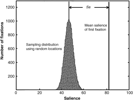
is usually high, especially for the first top fixations (i.e., k = 1, 2). The salience ![]() expected by chance is obtained by using randomly chosen locations in the corresponding saliency maps, which needs to be computed many times to generate a histogram distribution for the given database. The mean of the histogram distribution gives the average salience by chance. Assuming that the salience is scaled to range from 0 to 100, the difference between the mean salience obtained from the observed fixation locations and the mean salience expected by chance is referred as the chance-adjusted salience sa in [22]. It is clear that a larger chance-adjusted salience sa implies better performance of the given computational model. It is important to note that the chance-adjusted salience is not similar for different subjects and databases. This gives us a scheme to test the databases and can help to choose appropriate databases. As mentioned above, the mean salience of the first fixation significantly differs from mean salience with standard error by chance. A sketch map to explain the chance-adjusted salience between the mean salience of first fixation and the sampling distribution using random locations is shown in Figure 6.6.
expected by chance is obtained by using randomly chosen locations in the corresponding saliency maps, which needs to be computed many times to generate a histogram distribution for the given database. The mean of the histogram distribution gives the average salience by chance. Assuming that the salience is scaled to range from 0 to 100, the difference between the mean salience obtained from the observed fixation locations and the mean salience expected by chance is referred as the chance-adjusted salience sa in [22]. It is clear that a larger chance-adjusted salience sa implies better performance of the given computational model. It is important to note that the chance-adjusted salience is not similar for different subjects and databases. This gives us a scheme to test the databases and can help to choose appropriate databases. As mentioned above, the mean salience of the first fixation significantly differs from mean salience with standard error by chance. A sketch map to explain the chance-adjusted salience between the mean salience of first fixation and the sampling distribution using random locations is shown in Figure 6.6.
Figure 6.6 Sketch map of chance-adjusted salience between the mean salience of first fixation and the sampling distribution using random locations
Although the chance-adjusted salience is simple and can measure the agreement between human eye movements and model predictions, it is insufficient as it depends on subjects and databases. An improved analysis called normalized scanpath salience (NSS) has been proposed [23], in which each saliency map generated by the computational model is linearly normalized to have zero mean and unit standard deviation. A series of fixation locations along the subjects' scanpath are extracted from these normalized saliency maps. The average normalized salience value across all fixation locations is taken as the NSS. Due to pre-normalization of the saliency map, NSS values greater than zero suggest a greater correspondence than the expected value by chance. The improvement of pre-normalization makes the measure propitious to be compared across different subjects and image classes. The model with a higher NSS value should have better correspondence with human eye movement. The chance-adjusted salience and its improved version NSS, mainly use static saliency maps.
In 2005, Itti proposed a measure to quantify the degree to which human saccade matches a location of model-predicted saliency in video clips [25]. This measured index is known as the KL distance or as the KL score for the coherence with the ROC score. Since each frame in a video clip is presented only for a short period (10–20 ms), the scanpath only captures the most salient locations in each frame. It likely catches more bottom-up information in a single frame, and for the whole series of images or video clips it contains certain contents or scenarios and may have some top-down information. Hence, static saliency and dynamic saliency are not similar. Some definitions and KL score measures are introduced as follows.
Let SMh be the salient value at a position which is the maximum within nine pixels of the model's dynamic saliency map and SMr be the salient value at a random location which is randomly sampled within the model's dynamic saliency map with uniform probability in the same manner. Let SMmax be the maximum salient value over all the dynamic saliency maps. The ratios ![]() and
and ![]() of human and random saccades can be computed across all frames and subjects. Consequently, two probability distributions,
of human and random saccades can be computed across all frames and subjects. Consequently, two probability distributions, ![]() and
and ![]() , versus saccade amplitude are obtained in the form of histogram. The difference between the two histograms can be considered as a quantitative criterion to measure computational models.
, versus saccade amplitude are obtained in the form of histogram. The difference between the two histograms can be considered as a quantitative criterion to measure computational models.
As mentioned in Chapters 02 and 03, KL distance or KL score can quantify the difference in shape of probability density distributions. Denoting the probability density at variable k of the discrete distribution ![]() as ph(k) and the probability density of the distribution of histogram
as ph(k) and the probability density of the distribution of histogram ![]() as pr (k), the KL distance between human and random distributions is given as
as pr (k), the KL distance between human and random distributions is given as
where h, r are the probability distributions of ![]() and
and ![]() , respectively. It can be seen that the KL score is not symmetric: the ratio of
, respectively. It can be seen that the KL score is not symmetric: the ratio of ![]() is bigger than that of
is bigger than that of ![]() in general, and human probability density ph(k) is always put on the numerator of the logarithm in Equation 6.8.
in general, and human probability density ph(k) is always put on the numerator of the logarithm in Equation 6.8.
A larger KL score means that the computational model better matches human saccade targets that are different from random saccade targets.
Like chance-adjusted salience, the random saccade is repeated many times (e.g., 100 times), and generates the corresponding KL score at each instance. The standard deviation can be computed for each subgroup of saccades and then incorporated into the KL measure. For examples, in [30], the human-derived metric has a KL score of 0.679 ± 0.011 while the same for the entropy method is 0.151 ± 0.005. The surprise model has a KL score of 0.241 ± 0.006. It follows that the human-derived model performs the best (with the highest KL score), followed by the surprise model which in turn is better than the entropy method.