3.5 Attention Modelling Based on Information Maximizing

The BS model and its variations are based on feature integration theory, and the GBVS model with graph theory (which was discussed in the previous section) also works in a similar framework, since they all need low-level feature extraction and integration. Their feature maps obtained by using filters and contrast processes are based on explicit extraction of intensity, colour, orientation and so on, and then the final saliency map is a cross-feature integration. The BS model is very successful for simulating human attentional focus in numerous experiments including artificial and natural scenes.

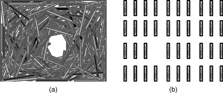
However, this definition of saliency based on local feature contrast may be somewhat questionable since some discarded regions from the feature extracting process in the BS model are possibly fixation locations [7, 34]. For instance, in Figure 3.10(a) many long bars of various colours with random orientation are almost stacked over the full scene except for a small homogeneous region and in Figure 3.10(b), in a regular bar array an absent region appears. Very often, these unique regions in their respective scenes are not detected by these filters in the BS model since there are no orientation or colour features in these regions, but their uniqueness attracts the fixation of human eyes. In the view of information theory, these unique regions have more information than other regions with repeating or random objects.

Figure 3.10 Examples failed in original BS

Also, in the feature extraction stage of the BS model, the filters extracting low-level features are fixed; for example four orientations are equally distributed between 0° and 180°, and are not adaptive to the scene's context. Actually, in the human brain, connections between these cells extracting features and their receptive fields, which the filters are emulating, are obtained by a learning process from input environment. The learning is to capture more useful information from the outside environment and discard the redundancy. Considering the properties of reducing information redundancy mentioned in Section 2.6.3 for both salient and feature filters' design criteria, the model of attention based on information maximization (AIM), is proposed by Bruce et al. [7, 34, 35]. From the view of the AIM model, the locations of attention focus in the input scene are just those places that include maximum information. In general, information is measures by entropy or self-information as defined in Section 2.6.3. The AIM model suggests a computational strategy to estimate self-information at each location, in which principal components analysis (PCA) and independent components analysis (ICA) are used as approaches to reduce redundancy and to achieve basis functions like simple cells' receptive fields. We will now introduce the idea of the AIM model, basis function attaining, self-information estimation and computational steps of the AIM model in detail.

3.5.1 The Core of the AIM Model

Figure 3.10 gives us a challenge: what is the saliency in scenes? Edges of objects or some locations with high contrast are often considered as salient regions in a scene but sometimes they may turn into inattentive areas. The reason is probably that there is significant redundancy in these inattentive areas. A game to guess the structure of an obscured region on a picture is proposed in [35]. Several observers are asked to guess the structure in covered patches of scene. These patches with repeated or similar structure to their surround may be guessed correctly with a high chance, and by contrast, the observers probably make mistakes in the covered patches if they are different from their surround. An example is shown in Figure 3.11(a) and (b) – an outdoor garden without and with obscured patches respectively. The obscured regions A and B (black solid circles) located in the blue sky and green lawn of Figure 3.11(b) are very easy to correctly estimate and the stonework (region C) that stands at the centre of the pool might be a difficult guess. The intuitional example means that the context of the neighbourhood is significant for measuring the salient location. This is equivalent to self-information related to each location and its context. Hence the AIM model suggests that the saliency of visual content may be equal to a measure of the information presented locally within a scene as defined by its surround [35].

Figure 3.11 An example of a guessing game (a) original image (b) the image with obscured patches

Self-information is a measure of the information content associated with the outcome of a random variable. The uncertainty of a random variable is often described as the probability by taking statistics over time or over a set. If the random variable is a probabilistic event x, the self-information of the event x depends only on the probability of that event associated with its context.

(3.34)

where p(x) is the probability of x. In the AIM model, the event can be regarded as a possible value that the observer guesses at a concealed image patch, and the context may be the patches surrounding the concealed image patch or even all the patches over whole scene. The unit of self-information depends on the base of logarithm used in its calculation. However, whatever unit you take it will not influence the result because saliency in a scene is relative. Evidently from Equation 3.34, the smaller probability with which the event does indeed occur, the larger the self-information associated with receiving the information. Self-information of a certain event is zero and the self-information of an event, that almost never happens, is equal to infinity. The measure of self-information is positive and additive. If an event A is composed of several independent events, then the amount of information that event A happens is equal to the sum of the information of the various independent events. Self-information is sometimes used as a synonym for entropy; that is entropy is the expected value of self-information (Equations 2.11 and 2.12 in Section 2.6.3). It is worth stressing that in the AIM model a local region (image patch) is considered as an event and the entropy or self-information is defined on the surround of local region under consideration.

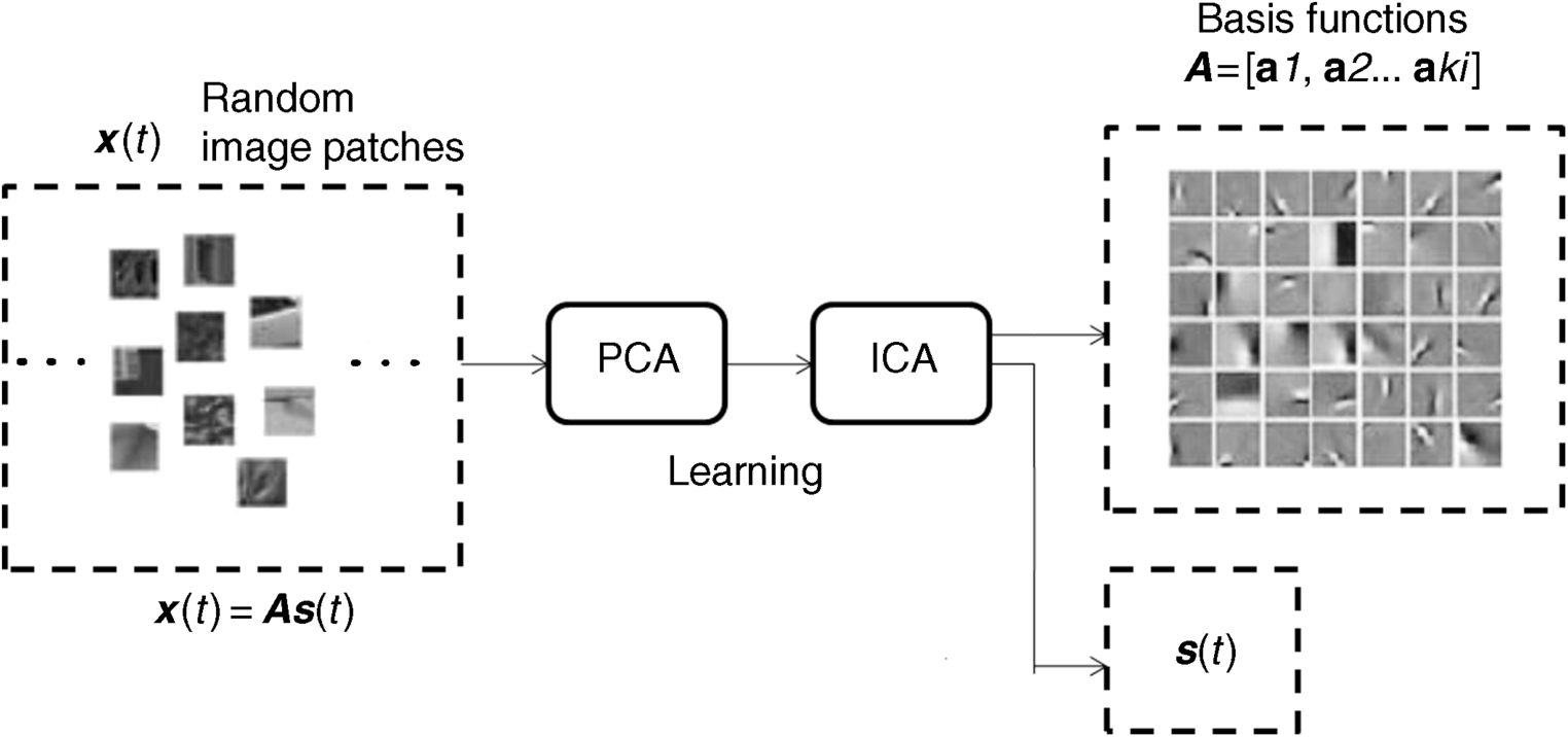
The next step is how to estimate the self-information of each image patch defined in its context. Even for a very small image patch, for example a 7 × 7 RGB patch, the estimation of probability density function residing in a very high dimensional space (49 × 3 dimensions) is very difficult and unfeasible, since it requires calculating a joint likelihood for a local window in RGB space based on measuring a mass of data, resulting in high computational complexity. Therefore, the dimensionality reduction adopted in many statistical applications is necessary. The AIM model employs ICA, introduced in Section 2.6.3, to reduce the dimensionality of the colour image patch. The basis functions of ICA are obtained by learning large numbers of patches, randomly sampled from thousands of natural images. An arbitrary test image patch can be described by the basis functions and the coefficient of each basis. Since the number of basis functions of ICA is far less than the dimension of an image patch, an image patch of high dimension can be represented by the coefficients of the ICA basis bank with low dimension, which reduces the computational complexity. On the other hand, these coefficients of the ICA basis bank are statistically independent, so the probability of an image patch that appeared is the product of the probability of these independent coefficients that respectively appeared. Therefore, it simplifies the computation of joint likelihood for self-information of the image patch under consideration. From the viewpoint of biology, we regard an image patch as a receptive field of simple cells in the primary visual cortex, and each basis of ICA is the weight vector to extract a related feature in the receptive field. Several cells share a receptive field to extract various features, and this is similar to filters of the feature extraction stage in the BS model. As the aforementioned difference from the BS model, these filters are not fixed and are obtained by learning from external stimuli. They include more general features such as spatial frequency, orientation, colour and position.

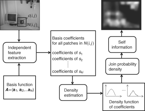
In summary, the AIM model consists of two parts: one is learning of basis functions by ICA and the other is self-information calculation of the image patch at each location defined on its surround. In the latter part, three steps are needed: (a) If the basis functions of ICA are given, the patch under consideration and its surround patches on the scene are projected onto each basis of ICA to get the related coefficients; (b) the probability density function of each coefficient defined on both the centre and surround patches is estimated by histogram or Gaussian kernel; (c) according to the probability density function of each coefficient and their independence, the self-information can be calculated by Equation 3.34 in each location on the scene.

Finally, the saliency map based on the AIM criterion is generated. The computational equation and drawing for each part and step are discussed below.

3.5.2 Computation and Illustration of Model

1. Preprocessing and learning of the ICA basis functions

Let denote a random vector with 3mn dimensions, where m and n are width and height of an image patch and the number 3 represents RGB space. The random variable of each dimension is denoted as for t = 1, 2, . . . T. The time T can be very large. For instance, in the AIM model a large number of local patches are randomly sampled from a set of 3600 natural images (100 image patches/per image) and formed 360,000 patches as a learning data set [35], so T = 360,000. Assuming that is generated as a linear mixture of independent components, if noise is ignored, Equation 2.16 in Section 2.6.3 can be rewritten as

(3.35)

We need to estimate the unknown random vector and mixing matrix A for a given , such that the components, of vector , are independent of each other. Here each column of matrix A, () is a spatiochromatic basis of ICA, since it may be an arbitrary kind of feature filter in spatial and chromatic spaces such as colour, spatial position, frequency, orientation and so on. So can be represented as

(3.36)

and

where the number of independent components ki 3mn, so the dimension of the original image patch is reduced, and the coefficients of spatiochromatic basis bank, are very sparse. It is noticed that the basis of ICA has the same dimension as and is fixed once the estimation is complete. In most algorithms of ICA, the estimation of independent components needs preprocessing to reduce computational complexity and to estimate the number of the basis. The PCA as the preprocessing stage can be first used to remove the second-order redundancy in random vector, . The operations of PCA, as mentioned in Section 2.6.3, are to compute covariance matrix of by using Equation 2.14, and then compute its eigenvalues and eigenvectors, and finally keep several eigenvectors corresponding to the largest eigenvalues. After PCA, the patch, , can be represented as a linear combination of several eigenvectors and related coefficients, and noise is wiped off in the original image patch.

In the AIM model, the authors applied the Jade ICA algorithm [36] to the chromatic patch set (360,000 patches) with the PCA preprocessing step retaining 95% energy (i.e., selecting ki largest eigenvalues such that their summation occupies 95% of the total eigenvalues' summation), and the ki eigenvectors corresponding to the ki largest eigenvalues as the dimensional number in the new space. For the patch with size of 31 × 31 chromatic pixels in original space, the dimensional number reduces to 54 and for the patch size of 21 × 21 chromatic pixels, ki = 25 in [35]. Although ICA can obtain both basis vectors and coefficients for each random chromatic patch from the learning data set, the main intent is to get basis vectors suitable for arbitrary natural images. These basis vectors of ICA are reformed to 2D form m × n (m = n in [35]) called basis functions in [35]. We may learn these basis functions by choosing different parameters in different applications, such as patch size, resulting dimension, learning set size T and ICA algorithms, before using the AIM model; however, basis functions proposed by [35, 37] on their website are ready and convenient to use. Figure 3.12 shows the framework to obtain spatiochromatic basis functions of ICA. It can be seen that these basis functions are like filters in the BS model; however, they become more diversified.

2. Independent feature extraction in a test patch

Suppose the basis vectors are available, that is the mixing matrix A consisting of basis vectors is available but it is not a square matrix due to reducing the dimension as shown in Equation 3.35. Consider an image patch centred at location (i, j) on a test scene, and rewrite it as a 3mn vector , where (i, j) is the coordinate of the centre pixel of the image patch. According to Equation 3.35, for the given learned mixing matrix A, the independent feature vector (coefficient vector), of , is defined as the product of the pseudo-inverse of mixing matrix A and .

(3.37)

where W is a un-mixing matrix, that is the pseudo-inverse of mixing matrix A, and the includes ki coefficients of ICA basis vectors:

For the colour patch with size of m × n pixels centred at an arbitrary (i, j) pixel location, the feature extraction is easily realized by Equation 3.37. The ki independent coefficients are just the features of the patch under consideration. The patches centred at the boundary or near boundary pixels of the input image are not considered due to having incomplete neighbours. It does not impact on the result much since the attention focus is often located in the middle part of an image. For special requirements, the border extending methods used in image processing techniques can undertake the processing of bordering patches.

3. Probability density function estimation

Consider one coefficient among the ki independent coefficients at the patch centred at location (i, j) and its neighbourhood patches. Without loss of generality, let be the coefficient of basis at the patch centred at (i, j) and let be its neighbour patches centred at , where represents neighbour pixels of (i, j). The probability density function for the set of coefficients, , centred at (i, j) and (u.v) corresponding to basis can be calculated by two methods, as follows.

One method is Gaussian kernel probability estimation [7]. Let the value of the independent coefficient be denoted by . An probability density estimation of based on a Gaussian window is given by

(3.38)

where denotes the contribution (weight) of the coefficient at coordinate (u, v) to the probability density estimation of the patch at coordinate (i, j), and is the value of the coefficient of the kth basis at coordinate (u, v). Parameter σ is the variance of Gaussian function. For the all ki independent coefficients at a patch with its neighbourhoods (surround), we can estimate the probability density function from Equation 3.38. To reduce the computational cost, Equation 3.38 can be implemented as a neural circuit (hardware) to compute them in parallel [7].

Another method is the histogram estimation with the number of bins chosen in value range of each independent coefficient defined on each patch and its local surround patches. It is a troublesome work since for each patch ki histograms need to be estimated. To save on computation, the authors in [7] have considered the extent of local surround (u, v) over the entire scene and each pixel location equally contributes to the estimation of the probability density function.

4. Self-information computation

When the probability density functions are obtained by the aforementioned methods, the probability density for a given image patch can be easily computed as follows. The value of each independent coefficient defined on patch is obtained by Step 2 and the probability density of the coefficient for the given value can be obtained from the probability density function. Since the probability densities of each independent coefficient are mutually independent, the joint probability density (joint likelihood) related to is written as

(3.39)

According to the definition of self-information (Equation 3.34) and Equation 3.39, the self-information related to patch is described as

(3.40)

The flowchart of the AIM model including the four steps above is shown in Figure 3.13.

In Figure 3.13, the left part of the figure is Step 2, where and represent the patch being considered and its neighbourhood at location (i, j), respectively. All possible patches centred at need to calculate ki coefficients through the basis function bank that has been learned from the database beforehand. The middle part and bottom right part are Step 3, where each of coefficients (s₁, s₂, . . . s_ki) is a coefficient set for the patches in and , and the top right part is Step 4.

As mentioned above, the location with a higher value of self-information has more information than those with lower values; in other words, the location with a higher value of self-information is more salient, because the structure in the patch with high self-information is seldom among its surround patches, which can pop out from its neighbourhood.

In summary, AIM modelling has four steps: (1) the basis functions are learned from chromatic patch database with randomly sampling; (2) for any input image, each pixel is regarded as the centre of a patch and the patch under consideration is projected onto the basis functions to obtain the independent coefficients (features); (3) with the surrounding (neighbouring) patches (including the patch itself), the probability density function is calculated for each independent coefficient; (4) self-information is calculated for each position and the saliency map is formed. The AIM model is a computational model and has been programmed in MATLAB® code [37].

In 1998, a result from [38] found that when ICA was used on natural image sequences, these ICA basis functions of natural image sequences are similar to simple cells in the V1 area. Hence, the AIM model can also be extended to video when ICA basis functions are based on spatiotemporal volumes [35]. In that case, the other steps (Steps 2–4) of the AIM model are the same, but they are based on 3D volumes, not 2D patches.

Figure 3.12 The framework for learning basis of ICA, here each basis of ICA, , is a recovered 2D colour patch. The learning basis set of x(t) is 360,000 image patches randomly sampled from 3600 nature images [35]

Figure 3.13 The flowchart of the AIM computational model