4.5 Pulsed Discrete Cosine Transform Approach

Visual attention computational models in the frequency domain have faster computational speed and better performance than models in the spatial domain. However, it is not clear why they can obtain the perfect salient locations in input scenes, and what their biological basis is. Since in our brain there is no mechanism similar to the Fourier transform, frequency domain models have no biological basis, though some simple cells in the primary visual cortex may extract frequency features from input stimuli. One idea to find why this, should come from the development of connected weights in a feed-forward neural network as proposed in [7, 46]. It is known that the connected weights between neurons in the human brain are commonly obtained by the Hebbian learning rule [47, 48], and a lot of previous studies have showed that single layer feed-forward neural network, when given large numbers of data by the Hebbian learning rule, can find the principal components of the input data [49, 50]. The adjustment of the connected weights between input and output neurons at the learning stage is similar to the development stage of the visual system. When the connections are nearly stable, the neural network behaves like a linear transform from input image to all its principal components. Principal components analysis (PCA), mentioned in Section 2.6.3, can capture the main information of the visual inputs which is probably related to the spatial frequency of the input image. A computational model based on PCA is proposed in [7] and [46], in which all the principal components are normalized to a constant value (one), by only keeping their signs. Since PCA is data dependent and its computation complexity is too high to be implemented in real time, a new consideration is that the PCA transform can be replaced by the discrete cosine transform in [7, 46], referred to as the pulse cosine transform (PCT). The approach based on the discrete cosine transform is data independent, and there are various fast algorithms for most image and video coding applications. Thus, PCT can calculate the saliency map easily and rapidly.

4.5.1 Approach of Pulsed Principal Components Analysis

Given an image with M × N pixels, we can rewrite it as an n-dimensional space (n = M × N). A vector in the n-dimensional space represents an image, which is inputted to a single-layer neural network. When a mass of images in a scene are continually inputted to the neural network, connections between input and neurons are adapted by the Hebbian rule, and finally these connections tend to become stable. The final connections of each neuron form another n-dimensional vector. Orthonormal processing of all connected vectors builds a new coordinate space and the connected weight vectors are called the basis of PCA [49, 50]. The neural network represents a linear transform from image coordinate axes to principal component coordinate axes that have the same number of dimensions as the input space. This linear transform is called Karhunen–Loève transform (KL transform in short or PCA). The output of each neuron in the neural network is a principal component of the input. It is worth noting that these principal components are uncorrelated to each other, so the KL transform produce optimally compact coding for images. As with other orthogonal transforms such as Fourier transform and discrete cosine transform, if all the principal components are reserved, the inverse KL transform can completely recover the original image. It has been shown that the principal components of natural images reflect the global features in the visual space, and all the redundancy reflected in the second-order correlations between pixels is captured by the transform [51].

An interesting result of PCA related to the power spectra of images is that when the statistical property of an image set is stationary, power spectral components of these images are uncorrelated to each other [51, 52]. The stationary statistics assumption may be reasonable for natural scenes since there are no special locations in an image where the statistics is different [52]. Therefore, for the case of stationary statistics, the amplitude spectrum maybe approximates to the principal components [51, 52]. Therefore we can use the same scheme to process the KL transform as in the frequency domain.

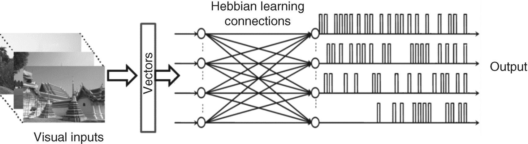
In order to simplify the computation, the learning stage of PCA is omitted and its basis vectors are obtained by using some efficient numerical methods such as eigenvalue decomposition or the QR algorithm (a matrix is decomposed as two matrices Q and R) method) [53]. If all the n basis vectors of PCA are available, for given image I with M × N pixels, the pulsed PCA approach will be implemented by the following four steps: (1) Reshape the 2D image into an n-dimensional vector as shown on the left of Figure 4.12. (2) Calculate KL transform by using basis vectors of PCA or input feed-forward neural network with known connected vectors (basis vectors of PCA), and then set all the coefficients of PCA to one, by only keeping the sign of these coefficients as the output of neural network in Figure 4.12 (binary code). (3) Take the inverse KL transform for the output and take the absolute value for the recovered image. (4) Post-process the recovered image by Gaussian filter to get the saliency map.

Figure 4.12 Neural network generating binary code, where connections are the basis vectors of PCA. The visual input is image sequences and output, normalized by a signum function, becomes a binary code (+1 is pulse and −1 is zero in the figure) [46]. Reprinted from Neurocomputing, 74, no. 11, Ying Yu, Bin Wang, Liming Zhang, ‘Hebbian-based neural networks for bottom-up visual attention and its applications to ship detection in SAR images’, 2008–2017, 2011, with permission from Elsevier

For a given input image I with M × N pixels, the computational equations for each step are illuminated as follows:

Step 1. Reshape 2D image to n-dimensional vector I ⇒ x, , n = M × N.

Step 2. Calculate KL transform of vector x and take the sign of each coefficient

(4.45)

where is an n × n PCA transformation matrix that comprises n principal basis vectors. The notation sign(.) is the signum function. The operation of Equation 4.45 produces binary code (1s and −1s), so when the video sequence inputs the neural network of Figure 4.12, the output of each neuron appears as a series of pulses: code 1s denotes pulse and code; −1s denotes no pulse as in Figure 4.12 for explicitly displaying.

Step 3. Do inverse KL transform of

(4.46)

where abs(.) is the absolute value function and x′ is the n-dimensional vector. Taking the absolute value of the inverse KL transform expresses the positive values on the saliency map. After a reshaped operation, the vector is rewritten as a 2D image I′: x′ ⇒ I′.

Step 4. Post-process the 2D image: I′ is convolved by a low-pass Gaussian filter for smoothing. The final saliency map is expressed as

(4.47)

where the power of I′, k, is an integer to enhance the salient regions. In other frequency domain models (SR, PFT and PQFT), k is selected as k = 2. For the pulsed PCA model, k can be chosen as any number other than 2. The symbol G in Equation 4.47 is the 2D low-pass Gaussian filter.

4.5.2 Approach of the Pulsed Discrete Cosine Transform

The pulsed PCA model probably has a little biological plausibility related to the Hebbian learning rule in the feed-forward neural network, but its computational complexity is high. Even though we use some efficient mathematical methods to calculate the PCA basis, for n = M × N size, it still works in a very high dimensional computational space (the size of matrix _L is (n × n) in Equations 4.45 and 4.46). Otherwise, as mentioned above, PCA is data dependent in technique, and its transform is influenced by the statistical properties of the learning dataset. Many studies have confirmed that the basis vectors of PCA probably resembles the basis vectors of the discrete cosine transform (DCT) [54, 55] under certain conditions (i.e., the training set has stable statistical properties and the number of training images or the size of the training set tends to infinity). Therefore, the KL transform in Equations 4.45 and 4.46 can be replaced by a DCT, while calculating the saliency map. This method is referred to as pulsed discrete cosine transform (PCT). For given input image I with M × N pixels, the 2D-discrete cosine transform (2D-DCT) for I and the inverse DCT are calculated by the following equations

(4.48)

(4.49)

where C_F(u, v) is the DCT coefficient located at (u, v), and I (x, y) is the pixel value at location (x, y) in the input image. PCT is similar to pulsed PCA, the main difference being that we only take the sign of the DCT coefficients (Equation 4.50), and then calculate the inverse DCT and take the absolute value (Equation 4.51).

(4.50)

(4.51)

where and are the DCT and inverse DCT(IDCT) matrices respectively. The final saliency map of the PCT approach 4.47 is:

The computation above is the same as the pulsed PCA, so here we rewrite Equation 4.47 as the saliency map of PCT.

DCT is one kind of frequency transform while the input image is symmetrically mapped to the sides of (−x) and (−y) axes. The even symmetry image is four times the size of the original images. It is known that the Fourier transform for the even symmetry image has a zero imaginary part (sinusoidal coefficients equal to zero). This implies that the phase spectrum , while the signs of the cosine coefficients are positive or negative. Since Equation 4.50 seems to take the phase spectrum of the Fourier transform from the even symmetry image with larger size, PCT is almost the same with PFT. However, the PCT approach is developed from the pulsed PCA model that provides a little biological basis for these frequency domain approaches.

In addition, the discrete cosine transform is commonly used in image and video coding in which several fast algorithms have been proposed for fast and easy implementation.

Experimental results in [7, 46] show that the PCT and pulsed PCA models have the same results in natural image sets and psychophysical patterns, but PCT is faster than the pulsed PCA approach.

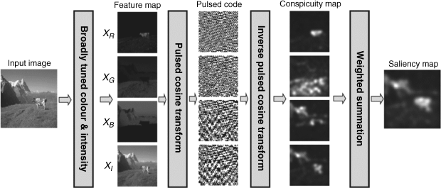
4.5.3 Multichannel PCT Model

Considering the feature integration theory, the multichannel model firstly computes the features for separate channels, and then combines them as whole. It is worth stating that the PCT approach does not adopt colour-opponent features, but only takes broadly tuned colour features as in [2], since sometimes colour-opponent features lose some information. For example, it probably cannot simultaneously detect the red target among the green distractors and the green target among the red distractors in the same red/green opponent channel. Let us consider four feature channels for a still image: one is the intensity feature and others are three colour features: broadly red, green and blue, that is similar to Equation 3.2. If r, g and b are the red, green and blue values in a colour image, and we denote the four features as X_I, X_R, X_G and X_B, we have

(4.52)

where [.]₊ denotes rectification, that is a negative value in square brackets is set to zero. To preserve the energy balance between all the feature channels, a weighted factor for each feature channel is calculated as

(4.53)

All feature channels are calculated by PCT above using Equations 4.48–4.51, respectively, and obtain conspicuity maps SM_I, SM_R, SM_G and SM_B. Then the combination is calculated as

(4.54)

The final saliency map is obtained by post-process of the 2D image SM (Equation 4.47). Figure 4.13 shows the flow chart of the multichannel PCT model.

Figure 4.13 Flow chart of the multichannel PCT model from original image (left) to saliency map (right). Note that the conspicuity maps and the saliency map are normalized for visibility [46]. Reprinted from Neurocomputing, 74, no. 11, Ying Yu, Bin Wang, Liming Zhang, ‘Hebbian-based neural networks for bottom-up visual attention and its applications to ship detection in SAR images’, 2008–2017, 2011, with permission from Elsevier

It has been shown in [7, 46] that the multichannel PCT model can obtain saliency maps in natural scenes and in psychophysical patterns which have similar or better performance than spatial models and PQFT.

In terms of speed, PCT has the same as PFT and is faster than SR and PQFT.

Since PCT and pulsed PCA adopt different colour features than PFT and PQFT approaches, and since they consider the weights in different channels, the performance of PCT is equivalent to or a little better than PQFT according to the test results with provided data sets in [7, 46]. Finally, PCT is programmable and easy to implement in MATLAB®, and it can be used in engineering applications.