3.1 Baseline Saliency Model for Images

The baseline salience (BS) model (referred to as Itti's model in some literature) refers to the classical bottom-up visual attention model for still images, proposed by Itti et al. [2], and its variations have been explored in [3–5, 11, 12]. Their core modules are shown in Figure 3.1.

Figure 3.1 The core of bottom-up visual attention models [2, 5] in the spatial (pixel) domain. © 1998 IEEE. Reprinted, with permission, from L. Itti, C. Koch, E. Niebur, ‘A model of saliency-based visual attention for rapid scene analysis’, IEEE Transactions on Pattern Analysis and Machine Intelligence, Nov. 1998

In Figure 3.1 the low-level features of an input still image for three channels (intensity, colour and orientation) are extracted and each channel is decomposed into a pyramid with nine scales. The centre–surround processing between different scales is performed to create several feature maps for each channel. Then fusing of across-scale and normalization for these channels produces three conspicuity maps. Finally, the three conspicuity maps are combined into a saliency map of the visual field. As mentioned above, the saliency map is the computational result of the attention model.

There are five characteristics of the core of this bottom-up visual attention model:

We will discuss the major ideas in [2, 3, 5, 11, 12] for processing intensity, colour and orientation features to derive the saliency map for an image.

3.1.1 Image Feature Pyramids

Intensity, colour and orientation are the features that attract human visual attention and their actual effects in a particular pixel or region under consideration (termed the centre) depend upon the feature contrast (rather than the absolute feature value) of this centre and its surroundings (termed the surround). The features in the surroundings can be approximated by low-pass filtered and the down-sampled versions of the feature images. Therefore, the extraction of various features is discussed first, followed by the feature pyramid generation.

For an RGB (red–green–blue) colour image, the intensity image p_I can first be computed from its three corresponding colour channels r, g and b at every pixel [2]:

(3.1)

where the dynamic range of p_I at every pixel is [0,1]. It should be noted here that the italic denotes scalar and the bold italic represents image (matrix or vector) in this book. For the colour space (corresponding to the colour perception mechanism in the human visual system (HVS) [13]) the colour antagonist is used here, and the red–green (RG) and blue–yellow (BY) opponent components need to be computed. Since the yellow colour with r = g = 1, b = 0 at a pixel is not propitious for the computation in r, g, b colour space (e.g., the yellow colour component in the case of pure red or pure green is not equal to zero), so broadly tuned colours: R(red), G(green), B(Blue), Y(Yellow) are created as [2]:

(3.2a)

(3.2b)

(3.2c)

(3.2d)

where i denotes the location of the ith pixel in the colour image, and symbol [·]₊ denotes rectification, that is a negative value in square brackets is set to zero. In addition, when p_Ii < 1/10, then R_i, G_i, B_i and Y_i are set to zero, because very low luminance is not perceivable by the HVS, and this is consistent with the threshold for guided search in the GS2 model as mentioned in Chapter 2. It can be seen from Equation 3.2 that for a pure red pixel in the input image (r = 1, b = 0, g = 0), the broadly tuned colour R_i = 3.0, G_i = B_i = Y_i = 0; for pure green or pure blue, only their corresponding broadly tuned colour, G_i or B_i, is equal to 3.0, and other colours are equal to zero. It is the same for a broadly tuned yellow pixel (r = g = 1, b = 0), and the broadly tuned colour Y_i = 3.0, R_i = G_i = 0.75 and B_i = 0. For a grey image (colour r, g and b are identity), all broadly tuned colours are equal to zero, which means there is no colour information in the image. Broadly tuned colour can keep in balance with the four kinds of colours. Other representations of broadly tuned colour are quite similar but here we do not introduce them one by one.

Since some colour detective cells in human vision are sensitive to the colour antagonist, the RG and BY opponent components for each pixel in a colour image are defined as the difference between two broadly tuned colours [2]:

(3.3a)

(3.3b)

Note that the subscript i of Equation 3.3 is omitted for simplicity. Here, balance colour opponents are created (p_RG = 3.0 or −3.0 for pure red or green, and p_BY = 3.0 or −3.0 for pure blue and yellow by using Equation 3.3). However, since the discrepancy of the computational results of Equation 3.3 for different colours (orange, magenta, cyan, etc.), the RG and BY opponent components are modified as [5]:

(3.4a)

(3.4b)

For the same reason for a broadly tuned colour, when max(r, g, b) < 1/10 at a pixel being considered (assuming a dynamic range of [0,1] for colour r, g and b), p_RG and p_BY are set to zero. In Equation 3.4, the broadly tuned colours do not need to be computed and this simplifies the system implementation, but as a method for opponent colour components, Equations 3.2 and 3.3 are still used in some models and applications.

Gaussian pyramids for p_I, p_RG and p_BY are built as p_I(d), p_RG(d) and p_BY(d), where d (d = 0,1, . . . , 8) denotes the scale of a pyramid, via Gaussian low-pass filtering and down-sampling progressively. As aforementioned, the bold italic represents image (matrix or vector). The higher the scale index d is, the smaller the image size becomes; d = 0, representing the original image size, and d = 8, representing the 1 : 256 down-sampling along each dimension; in other words, the number of pixels when d = 8 is (1/256)² of that when d = 0. At the d-th scale, the image is first low-pass filtered to prepare for down-sampling into the (d + 1)-th scale [2], as illustrated with the following equation:

(3.5a)

(3.5b)

(3.5c)

where low-pass filtering is done using a separable Gaussian filter kernel G_a; if the 1D separable Gaussian filter kernel is chosen to be [1/16 1/4 3/8 1/4 1/16], then G_a is a 5 × 5 Gaussian kernel: G_a = [1/16 1/4 3/8 1/4 1/16]^T [1/16 1/4 3/8 1/4 1/16]; symbol * denotes the convolution operator; the superscript ‘0’ represents the filtering results. Afterwards down-sampling is performed to create a sub-image for each pyramid scale:

(3.6a)

(3.6b)

(3.6c)

From Equation 3.6, there are nine different sizes of intensity images corresponding to nine resolutions, and these images are called the intensity pyramid; since there are nine images for each colour-opponent feature, there are 18 images in the two colour pyramids in total, which are illustrated in Figure 3.1.

As for orientations, Gabor filters are utilized to derive orientated pyramids [14] from p_I:

(3.7)

where d is the scale of the pyramids, being the same as the cases of P_I(d), P_RG(d) and P_BY(d), d = [0,1, . . . 8], and is the real component of a simple, symmetric Gabor filter [14], its element value at location (x, y) for orientation θ being

(3.8)

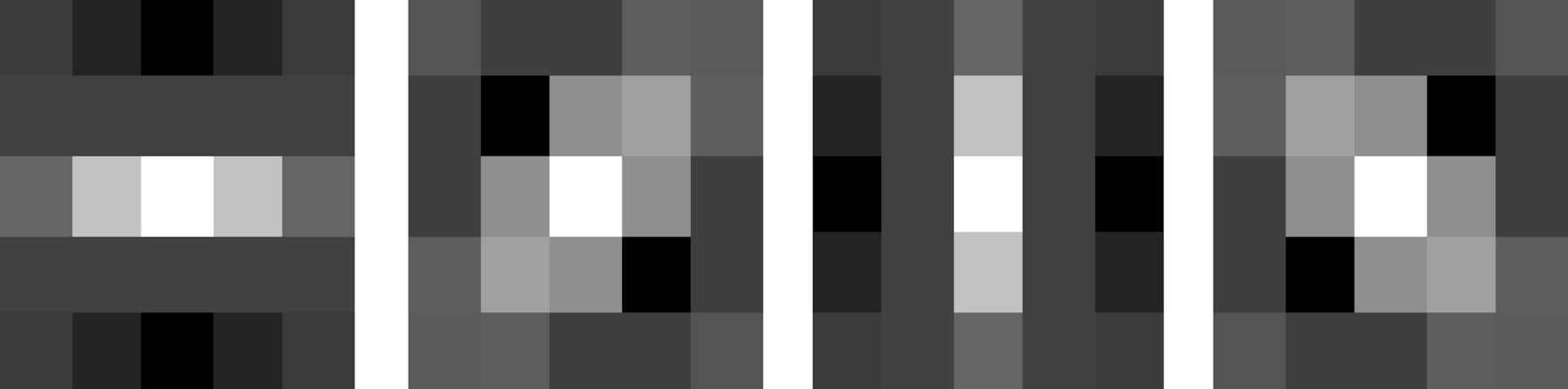
where the origin of x and y is at the centre of the kernel; the kernel size can be 5 × 5 [14] (or a more comprehensive Gabor function with a bigger kernel size, as in [5]); four orientations are evaluated, so θ = 0°, 45°, 90° and 135° as shown in Figure 3.2. There are totally 36 images in orientation pyramids with nine scales for each orientation after Gabor filtering.

Figure 3.2 An example of a simple kernel of Gabor filter defined in Equation 3.8 with θ = 0°, 45°, 90° and 135°, respectively, when the kernel size is 5 × 5

3.1.2 Centre–Surround Differences

After building the feature pyramids p_I, p_RG, p_BY and p_o as above, the centre–surround differences can be generated for feature maps, which simulate the difference of Gaussian (DoG) filters in ganglion cells of the retina as mentioned in Section 2.5.3.

Intensity feature maps in Figure 3.1 are obtained by utilizing centre–surround differences for various centre and surround scales [2]. The difference between finer and coarser scales can be computed by interpolating a coarser scale to a finer scale for point-by-point subtraction between two intensity images. Centre scales are selected as q {2, 3, 4}, and the surround scales are defined as s = q + δ, where δ {3, 4}. Therefore, the intensity feature map for centre scale q and surround scale s is acquired as

(3.9a)

where is the interpolated version of p_I(s) to scale q. Similarly, we can have the centre–surround differences for colour-opponent p_RG, p_BY and orientation p_O:

(3.9b)

(3.9c)

(3.9d)

Please note that the scale for the resultant p_I(q, s), p_RG(q, s), p_BY(q, s) and p_o(q, s, θ) is q (q {2, 3, 4}). In essence, Equation 3.9 evaluates pixel-by-pixel contrast for a feature, since the feature at scale q represents the local information while that at scale s (s > q) approximates the surroundings. With one intensity channel, two colour channels and four orientation channels (θ = 0°, 45°, 90° and 135°), there are a total of 42 feature maps computed: 6 for intensity, 12 for colour and 24 for orientation. The centre–surround difference is shown in the middle part of Figure 3.1.

3.1.3 Across-scale and Across-feature Combination

Normalization is the property in the human visual perception as mentioned in Section 2.5.2. After centre–surround operation, all 42 feature maps are normalized via the function represented by N(·) as defined with the following procedures:

1. Normalize the values of a map to a fixed-range [0 . . . M_l] to avoid the modality-dependent amplitude differences.

2. Find its global maximum M_l and compute the average of its other local maxima; globally multiply the map by .

As a consequence, when the differences in a map are big (i.e., () is big), the differences are promoted by N(·); otherwise, they (corresponding to homogenous areas in the map) are suppressed.

Cross-scale combination is performed as follows, to derive the intensity, colour and orientation conspicuity maps respectively:

(3.10a)

(3.10b)

(3.10c)

The summation defined with Equations 3.10 is carried out at Scale 4, so down-sampling is needed for the p_I(q, s), p_RG(q, s), p_BY(q, s) and p_O(q, s, θ) when q is 2 and 3. This cross-scale summation accommodates different sizes of objects that attract attention in an image. After computation of Equations 3.10a, three conspicuity maps corresponding to intensity, colour and orientations channels are generated. It should be noticed that the size of conspicuity map is at Scale 4, that is the number of pixels on each conspicuity map is 1/(16)² of the original image. For example, for an input image with 640 × 480 pixels its size for conspicuity maps is 40 × 30 pixels.

The final saliency map of the image is obtained by a cross-feature summation [2]:

(3.11)

The value of each pixel on the saliency map (SM) reflects the salient level corresponding to a region of the input image, which will guide eye movement, object search and so on.

In summary, the BS model not only adopts the relevant psychological conceptions such as parallel multichannel feature extraction and feature integration in FIT and GS, but also considers other physiological properties, for instance, colour-opponent components features, Gabor orientation feature extraction, centre–surround difference simulating DoG filters in ganglion cells of retina, normalization and multiple sizes processing simulating the receptive field with different sizes. Consequently, the model is biologically motivated and can simulate most phenomena of psychological testing shown in Chapter 2. In addition, all the processes in the model have explicit computational formulations (Equations 3.1–3.11), and can be easily realized in computers (e.g., with the neuromorphic vision toolkit (NVT) in C++ [15]).