Arbitrage Pricing: Finite-State Models

SERGIO M. FOCARDI, PhD

Partner, The Intertek Group

FRANK J. FABOZZI, PhD, CFA, CPA

Professor of Finance, EDHEC Business School

The principle of absence of arbitrage or the no-arbitrage principle is perhaps the most fundamental principle of finance theory. In the presence of arbitrage opportunities, there is no trade-off between risk and returns because it is possible to make unbounded risk-free gains. The principle of absence of arbitrage is fundamental for understanding asset valuation in a competitive market. This entry discusses arbitrage pricing in a finite-state, discrete-time setting. However, it is important to note that there are well-known limits to arbitrage, first identified by Shleifer and Vishny (1997), resulting from restrictions imposed on rational traders and, as a result, pricing inefficiencies may exist for a period of time.

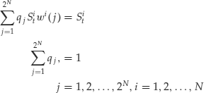
THE ARBITRAGE PRINCIPLE

Let’s begin by defining what is meant by arbitrage. In its simple form, arbitrage is the simultaneous buying and selling of an asset at two different prices in two different markets. The arbitrageur profits without risk by buying cheap in one market and simultaneously selling at the higher price in the other market. Such opportunities for arbitrage are rare. In fact, a single arbitrageur with unlimited ability to sell short could correct a mispricing condition by financing purchases in the underpriced market with proceeds from short sales in the overpriced market. This means that riskless arbitrage opportunities are short-lived.

Less obvious arbitrage opportunities exist in situations where a package of assets can produce a payoff (return) identical to an asset that is priced differently. This arbitrage relies on a fundamental principle of finance called the law of one price, which states that a given asset must have the same price regardless of the location where the asset is traded and the means by which one goes about creating that asset. The law of one price implies that if the payoff of an asset can be synthetically created by a package of assets, the price of the package and the price of the asset whose payoff it replicates must be equal.

When a situation is discovered whereby the price of the package of assets differs from that of an asset with the same payoff, rational investors will trade these assets in such a way so as to restore price equilibrium. This market mechanism is founded on the fact that an arbitrage transaction does not expose the investor to any adverse movement in the market price of the assets in the transaction.

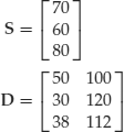
For example, consider how we can produce an arbitrage opportunity involving three assets A, B, and C. These assets can be purchased today at the prices shown below, and can each produce only one of two payoffs (referred to as State 1 and State 2) a year from now:

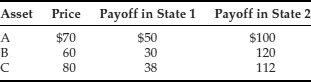
While it is not obvious from the data presented above, an investor can construct a portfolio of assets A and B that will have the identical payoff as asset C in both State 1 and State 2. Let wA and wB be the proportion of assets A and B, respectively, in the portfolio. Then the payoff (i.e., the terminal value of the portfolio) under the two states can be expressed mathematically as follows:

• If State 1 occurs: $50 wA+$ 30 wB
• If State 2 occurs: $100 wA+$ 120 wB

We create a portfolio consisting of A and B that will reproduce the payoff of C regardless of the state that occurs one year from now. Here is how: For either condition (State 1 and State 2), we set the payoff of the portfolio equal to the payoff for C as follows:

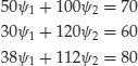
• State 1: $50 wA+$ 30 wB = $ 38
• State 2: $100 wA+$ 120 wB = $ 112

We also know that wA+wB = 1. If we solved for the weights for wA and wB that would simultaneously satisfy the above equations, we would find that the portfolio should have 40% in asset A (i.e., wA = 0.4) and 60% in asset B (i.e., wB = 0.6). The cost of that portfolio will be equal to

Our portfolio (i.e., package of assets) comprised of assets A and B has the same payoff in State 1 and State 2 as the payoff of asset C. The cost of asset C is $80 while the cost of the portfolio is only $64. This is an arbitrage opportunity that can be exploited by buying assets A and B in the proportions given above and shorting (selling) asset C.

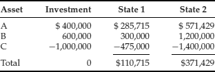
For example, suppose that $1 million is invested to create the portfolio with assets A and B. The $1 million is obtained by selling short asset C. The proceeds from the short sale of asset C provide the funds to purchase assets A and B. Thus, there would be no cash outlay by the investor. The payoffs for States 1 and 2 are shown below:

ARBITRAGE PRICING IN A ONE-PERIOD SETTING

We can describe the concepts of arbitrage pricing in a more formal mathematical context. It is useful to start in a simple one-period, finite-state setting as in the example of the previous section. This means that we consider only one period and that there is only a finite number M of states of the world. In this setting, asset prices can assume only a finite number of values.

The assumption of finite states is not as restrictive as it might appear. In practice, security prices can only assume a finite number of values. Stock prices, for example, are not real numbers but integer fractions of a dollar. In addition, stock prices are nonnegative numbers and it is conceivable that there is some very high upper level that they cannot exceed. In addition, whatever simulation we might perform is a finite-state simulation given that the precision of computers is finite.

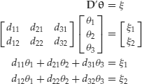
The finite number of states represents uncertainty. There is uncertainty because the world can be in any of the M states. At time 0 it is not known in what state the world will be at time 1. Uncertainty is quantified by probabilities but a lot of arbitrage pricing theory can be developed without any reference to probabilities. Suppose there are N securities. Each security i pays dij number of dollars (or of any other unit of account) in each state of the world j. The payoff of each security need not be a positive number. For instance, a derivative instrument might have negative payoffs in some states of the world. Therefore, in a one-period setting, the securities are formally represented by an N× M matrix where the dij entry is the payoff of security i in state j. The matrix D can also be written as a set of N row vectors:

where the M-vector di represents the payoffs of security i in each of the M states.

Each security is characterized by a price S. Therefore, the set of N securities is characterized by an N-vector S and an N× M matrix D. Suppose, for instance, there are two states and three securities. Then the three securities are represented by

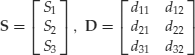
Every row of the D matrix represents one security, every column one state. Note that in a one-period setting, prices are defined at time 0 while payoffs are defined at time 1. There is no payoff at time 0 and there is no price at time 1. A portfolio is represented by an N-vector of weights . In our example of a market with two states and three securities, a portfolio is a 3-vector:

The market value of a portfolio at time 0 is a scalar given by the scalar product:

Its payoff at time 1 is the M-vector:

The price of a security and the market value of a portfolio can be a negative number. In the previous example of a two-state, three-security market we obtain

Let’s introduce the concept of arbitrage in this simple setting. As we have seen, arbitrage is essentially the possibility of making money by trading without any risk. Therefore, we define an arbitrage as any portfolio θ that has a negative market value and a nonnegative payoff or, alternatively, a nonpositive market value and a positive payoff .

State Prices

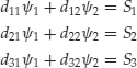
Next we define state prices. A state-price vector is a strictly positive M-vector such that security prices can be written as . In other words, given a state-price vector, if it exists, security prices can be recovered as a weighted average of the securities’ payoffs, where the state-price vector gives the weights. In the previous two-state, three-security example we can write:

Given security prices and payoffs, state prices can be determined solving the system:

This system admits solutions if and only if there are two linearly independent equations and the third equation is a linear combination of the other two. Note that this condition is necessary but not sufficient to ensure that there are state prices as state prices must be strictly positive numbers.

A portfolio is characterized by payoffs . Its price is given, in terms of state prices, by: .

It can be demonstrated that there is no arbitrage if and only if there is a state-price vector. The formal demonstration is quite complicated given the inequalities that define an arbitrage portfolio. It hinges on the separating hyperplane theorem, which says that, given any two convex disjoint sets in RM, it is possible to find a hyperplane separating them. A hyperplane is the locus of points xi that satisfy a linear equation of the type:

Intuitively, however, it is clear that the existence of state prices ensures that the law of one price introduced in the previous section is automatically satisfied. In fact, if there are state prices, two identical payoffs have the same price, regardless of how they are constructed. This is because the price of a security or of any portfolio is univocally determined as a weighted average of the payoffs, with the state prices as weights.

Risk-Neutral Probabilities

Let’s now introduce the concept of risk-neutral probabilities. Given a state-price vector, consider the sum of its components . Normalize the state-price vector by dividing each component by the sum . The normalized state-price vector

is a set of positive numbers whose sum is one. These numbers can be interpreted as probabilities. They are not, in general, the real probabilities associated with states. They are called risk-neutral probabilities. We can then write

We can interpret the above relationship as follows: The normalized security prices are their expected payoffs under these special probabilities. In fact, we can rewrite the above equation as

where expectation is taken with respect to risk-neutral probabilities. In this case, security prices are the discounted expected payoffs under these special risk-neutral probabilities.

Suppose that there is a portfolio such that . This portfolio can be one individual risk-free security. As we have seen above, , which implies that is the discount on riskless borrowing.

Complete Markets

Let’s now define the concept of complete markets, a concept that plays a fundamental role in finance theory. In the simple setting of the one-period finite-state market, a complete market is one in which the set of possible portfolios is able to replicate an arbitrary payoff. Call span(D) the set of possible portfolio payoffs, which is given by the following expression:

A market is complete if span(D) = RM.

A one-period finite-state complete market is one where the equation

always admits a solution. Recall from matrix algebra that this is the case if and only if the rank of D is M. This means that there are at least M linearly independent payoffs—that is, there are as many linearly independent payoffs as there are states. Let’s write down explicitly the system in the two-state, three-security market.

This system of linear equations admits solutions if and only if the rank of the coefficient matrix is 2. This condition is not verified, for example, if the securities have the same payoff in each state. In this case, the relationship must always be verified. In other words, the three securities can only replicate portfolios that have the same payoff in each state.

In this simple setting it is easy to associate risk-neutral probabilities with real probabilities. In fact, suppose that the vector of real probabilities p is associated to states so that pi is the probability of the i-th state. For any given M-dimensional vector x, we write its expected value under the real probabilities as

It can be demonstrated that there is no arbitrage if and only if there is a strictly positive M-vector such that: . Any such vector is called a state-price deflator. To see this point, define

Prices can then be expressed as

which demonstrates that .

We can now specialize the above calculations in the numerical case of the previous section. Recall that in the previous section we gave the example of three securities with the following prices and payoffs expressed in dollars:

We first compute the relative state prices:

Solving the first two equations, we obtain

However, the third equation is not satisfied by these values for the state prices. As a consequence, there does not exist a state-price vector, which confirms that there are arbitrage opportunities as observed in the first section.

Now suppose that the price of security C is $64 and not $80. In this case, the third equation is satisfied and the state-price vector is the one shown above. Risk-neutral probabilities can now be easily computed. Here is how. First sum the two state prices: 4/5+3/10 = 11/10 to obtain

and consequently the risk-neutral probabilities:

Risk-neutral probabilities sum to one while state prices do not. We can now check if our market is complete. Write the following equations:

The rank of the coefficient matrix is clearly 2 as the determinant of the first minor is different from zero:

Our sample market is therefore complete and arbitrage-free. A portfolio composed of the first two securities can replicate any payoff and the third security can be replicated as a portfolio of the first two.

ARBITRAGE PRICING IN A MULTIPERIOD FINITE-STATE SETTING

The above basic results can be extended to a multiperiod finite-state setting using probabilistic concepts. The economy is represented by a probability space where Ω is the set of possible states, is the algebra of events (recall that we are in a finite-state setting and therefore there are only a finite number of events), and P is a probability function. As the number of states is finite, finite probabilities are defined for each state. There is only a finite number of dates from 0 to T.

Propagation of Information

The propagation of information is represented by a filtration that, in the finite case, is equivalent to an information structure It. The latter is a discrete, hierarchical organization of partitions It with the following properties:

and, in addition, given any two sets , with h>k, either their intersection is empty or . In other words, the partitions become more refined with time.

Each security i is characterized by a payoff process dit and by a price process Sit. In this finite-state setting, dit and Sit are discrete variables that, given that there are M states, can be represented by M-vectors and where and are, respectively, the payoff and the price of the i-th asset at time and in state . All payoffs and prices are stochastic processes adapted to the filtration . Given that dit and Sit are adapted processes in a finite probability space, they have to assume a constant value on each partition of the information structure It. It is convenient to introduce the following notation:

where and represent the constant values that the processes dit and Sit assume on the states that belong to the sets of each partition It. There is M0 = 1 value for and , Mt values for and and MT = M values for and . The same notation and the same consideration can be applied to any process adapted to the filtration .

Trading Strategies

We have to define the meaning of trading strategies in this multiperiod setting. A trading strategy is a sequence of portfolios θ such that is the portfolio held at time t after trading. To ensure that there is no anticipation of information, each trading strategy θ must be an adapted process. The payoff generated by a trading strategy is an adapted process with the following time dynamics:

An arbitrage is a trading strategy whose payoff process is nonnegative and not always zero. In other words, an arbitrage is a trading strategy that is never negative and which is strictly positive for some instants and some states. Note that imposing the condition that payoffs are always nonnegative forbids any initial positive investment that is a negative payoff.

A consumption process is any nonnegative adapted process. Markets are said to be complete if any consumption process can be obtained as the payoff process of a trading strategy with some initial investment. Market completeness means that any nonnegative payoff process can be replicated with a trading strategy.

State-Price Deflator

We will now extend the concept of state-price deflator to a multiperiod setting. A state-price deflator is a strictly positive adapted process such that the following set of M equations hold:

In other words, a state-price deflator is a strictly positive process such that prices Sit are random variables equal to the conditional expectation of discounted payoffs with respect to the filtration . As noted above, in this finite-state setting a filtration is equivalent to an information structure It. Note that in the above stochastic equation—which is a set of M equations, one for each state, the term on the left, the prices Sit, is an adapted process that, as mentioned, assumes constant values on each set of the partition It. The term on the right is a conditional expectation multiplied by a factor . The process is adapted by definition and, therefore, assumes constant values on each set of the partition It.

In this finite setting, conditional expectations are expectations computed with conditional probabilities. Conditional expectations are adapted processes. Therefore they assume one value at t = 0, Mj values for t = j, and M values at the last date.

To illustrate the above, let’s write down explicitly the above equation in terms of the notation and . Note first that

Given that the probability space is finite,

As we defined , the previous equation becomes

if .

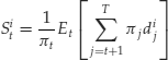
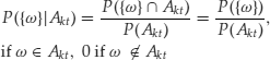
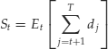
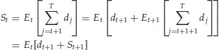
Pricing Relationships

We can now write the pricing relationship as follows:

The above formulas generalize to any trading strategy. In particular, if there is a state-price deflator, the market value of any trading strategy is given by

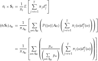
It is possible to demonstrate that the payoff-price pair (dit, Sit) admits no arbitrage if and only if there is a state-price deflator. These concepts and formulas generalize those of a one-period setting to a multiperiod setting.

Given a payoff-price pair (dit, Sit) it is possible to compute the stateprice deflator, if it exists, from the previous equations. In fact, it is possible to write a set of linear equations in the for each period. One can proceed backward from the period T to period 1 writing a homogeneous system of linear equations. As the system is homogeneous, one of the variables can be arbitrarily fixed; for example, the initial value can be assumed equal to 1. If the system admits nontrivial solutions and if all solutions are strictly positive, then there are state-price deflators.

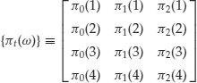
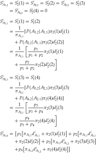
To illustrate the above, let’s write down explicitly the previous formulas for prices, extending the example of the previous section to a two-period setting. We assume there are three securities and two periods, that is, three dates (0,1,2) and four states, indicated with the integers 1,2,3,4, so that {1,2,3,4}. Assume that the information structure is given by the following partitions of events:

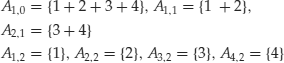
where we use + to indicate logical union, so that, for example, is the event formed by states 1 and 2. The interpretation of the above notation is the following. At time zero the world can be in any possible state, that is, the securities can take any possible path. Therefore the partition at time zero is formed by the event . At time 1, the set of states is partitioned into two mutually exclusive events, or . At time 2 the partition is formed by all individual states. Note that this is a particular example; different partitions would be logically admissible.

Figure 1 An Information Structure with Four States and Three Dates

Figure 1 represents the above structure. Each security is characterized by a price process and a payoff process adapted to the information structure. Each process is a collection of three discrete random variables indexed with the time indexes 0,1,2. Each discrete random variable is a 4-vector as it assumes as many values as states. However, as processes are adapted, they must assume the same value on each partition of the information structure. Note also that payoffs are zero at date zero and prices are zero at date 2. Therefore, in this example, we can put together these vectors in two 3× 4 matrices for each security as follows

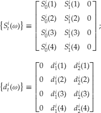
The following relationships hold:

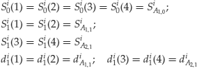
where, as above, is the price of security i in state at moment t and is the payoff of security i in state at time t with the restriction that processes must assume the same value on partitions. This is because processes are adapted to the information structure so that there is no anticipation of information. One must not be able to discriminate at time 0 events that will be revealed at time 1 and so on.

Observe that there is no payoff at time 0 and no price at time 2 and that the payoffs at time 2 have to be intended as the final liquidation of the security as in the one-period case. Payoffs at time 1, on the other hand, are intermediate payments. Note that the number of states is chosen arbitrarily for illustration purposes. Each state of the world represents a path of prices and payoffs for the set of three securities. To keep the example simple, we assume that of all the possible paths of prices and payoffs only four are possible.

The state-price deflator can be represented as follows:

A probability is assigned to each of the four states of the world. The probability of each event is simply the sum of the probabilities of its states. We can write down the formula for security prices in this way:

Table 1 Conditional Probabilities

These equations illustrate how to compute the state-price deflator knowing prices, payoffs, and probabilities. They form a homogeneous system of linear equations in , .

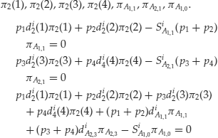
Substituting, we obtain

This homogeneous system must admit a strictly positive solution to yield a state-price deflator. There are seven unknowns. However, as the system is homogeneous, if nontrivial solutions exist, one of the unknowns can be arbitrarily fixed, for example . Therefore, six independent equations are needed. Each asset provides two conditions, so a minimum of three assets are needed.

To illustrate the point, we assume that all states (which are also events in this discrete example) have the same probability 0.25. Thus the events of the information structure have the following probabilities: the single event at time zero has probability 1, the two events at time 1 have probability 0.5, and the four events at time 2 coincide with individual states and have probability 0.25. Conditional probabilities are shown in Table 1.

For illustration purposes, let’s write the following matrices for payoffs for each security at each date in each state:

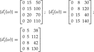
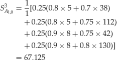
We will assume that the state-price deflator is the following given process:

Each price is computed according to the previous equations. For example, calculations related to asset 1 are as follows:

With the above equations we computed prices from payoffs and state-price deflators. If prices and payoffs were given, we could compute state-price deflators from the homogeneous system for state prices established above. Suppose that the following price processes were given:

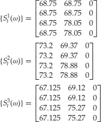
We could then write the following system of equations to compute state-price deflators:

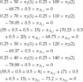
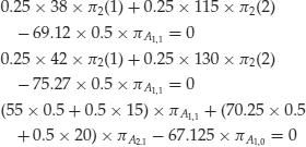
It can be verified that this system, obviously, is solvable and returns the same state-price deflators as in the previous example.

Equivalent Martingale Measures

We now introduce the concept and properties of equivalent martingale measures. This concept has become fundamental for the technology of derivative pricing. The idea of equivalent martingale measures is the following. A martingale is a process Xt such that at any time t its conditional expectation at time s, s>t coincides with its present value: Xt = Et[Xs]. In discrete time, a martingale is a process such that its value at any time is equal to its conditional expectation one step ahead. In our case, this principle can be expressed in a different but equivalent way by stating that prices are the discounted expected values of future payoffs. The law of iterated expectation then implies that price plus payoff processes are martingales.

In fact, assume that we can write

then the following relationship holds:

Given a probability space, price processes are not, in general, martingales. However it can be demonstrated that, in the absence of arbitrage, there is an artificial probability measure in which all price processes, appropriately discounted, become martingales. More precisely, we will see that in the absence of arbitrage there is an artificial probability measure Q in which the following discounted present value relationship holds:

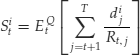
We can rewrite this equation explicitly as follows:

which shows that the discounted price plus payoff process is a martingale. The terms on the left are the price processes, the terms on the right are the conditional expectations under the probability measure Q of the payoffs discounted with the risk-free payoff.

The measure Q is a mathematical construct. The important point is that this new probability measure can be computed either from the real probabilities if the state-price deflators are known or directly from the price and payoff processes. This last observation illustrates that the concept of arbitrage depends only on the structure of the price and payoff processes and not on the actual probabilities. As we will see later in this entry, equivalent martingale measures greatly simplify the computation of the pricing of derivatives.

Let’s assume that there is short-term risk-free borrowing in the sense that there is a trading strategy able to pay for any given interval (t, s) one sure dollar at time s given that has been invested at time t. Equivalently, we can define for any time interval (t, s) the payoff of a dollar invested risk-free at time t as .

We now define the concept of equivalent probability measures. Given a probability measure P the probability measure Q is said to be equivalent to P if both assign probability zero to the same events. An equivalent probability measure Q is an equivalent martingale measure if all price processes discounted with Ri,j become martingales. More precisely, Q is an equivalent martingale measure if and only if the market value of any trading strategy is a martingale:

Risk-Neutral Probabilities

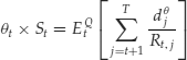
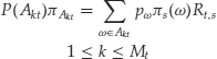
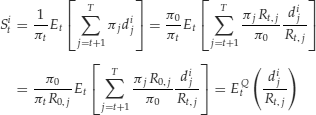
Probabilities computed according to the equivalent martingale measure Q are the risk-neutral probabilities. Risk-neutral probabilities can be explicitly computed. Here is how. Call the risk-neutral probability of state ω. Let’s write explicitly the relationship

as follows:

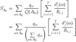
The above system of equations determines the risk-neutral probabilities. In fact, we can write, for each risky asset, Mt linear equations, where Mt is the number of sets in the partition It plus the normalization equation for probabilities. From the above equation, one can see that the system can be written as

This system might be determined, indetermined, or impossible. The system will be impossible if there are arbitrage opportunities. This system will be indetermined if there is an insufficient number of securities. In this case, there will be an infinite number of equivalent martingale measures and the market will not be complete.

Now consider the relationship between risk-neutral probabilities and state-price deflators. Consider a probability measure P and a nonnegative random variable Y with expected value on the entire space equal to 1. Define a new probability measure as Q(B) = E[1BY] for any event B and where 1B is the indicator function of the event B. The random variable Y is called the Radon-Nikodym derivative of Q and it is written

It is clear from the definition that P and Q are equivalent probability measures as they assign probability zero to the same events. Note that in the case of a finite-state probability space the new probability measure is defined on each state and is equal to

Suppose is a state-price deflator. Let Q be the probability measure defined by the Radon-Nikodym derivative:

The new state probabilities under Q are the following:

Define the density process for Q as . As is an adapted process, we can write:

As is the payoff at time s of one dollar invested in a risk-free asset at time t, s>t, we can then write the following equation:

Therefore,

Substituting in the previous equation, we obtain, for each interval (t, T),

which we can rewrite in the usual notation as

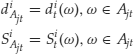
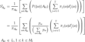
We can now state the following result. Consider any -measurable variable xj. This condition can be expressed equivalently stating that xj assumes constant values on each set of the partition Ij. Then the following relationship holds:

To see this, consider the following demonstration, which hinges on the fact that xj assumes a constant value on each Ahj and, therefore, can be taken out of sums. In addition, as demonstrated above, from

the following relationship holds:

Let’s now apply the above result to the relationship:

We have thus demonstrated the following results: There is no arbitrage if and only if there is an equivalent martingale measure. In addition, is a state-price deflator if and only if an equivalent martingale measure Q has the density process defined by

In addition, it can be demonstrated that, if there is no arbitrage, markets are complete if and only if there is a unique equivalent martingale measure.

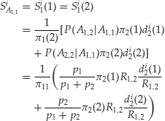
To illustrate the above we now proceed to detail the calculations for the previous example of three assets, three dates, and four states. Let’s first write the equations for the risk-free asset:

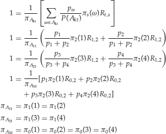
We can now rewrite the pricing relationships for the other risky assets as follows:

At date 2, prices are zero: Si2 = 0.

At date 1, the relationship

holds. In fact, we can write the following:

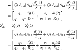
At date 0, the relationship

holds. In fact we can write the following:

The value of a derivative instrument might depend on the path of its past values. Consider a lookback option on a stock—that is, a derivative instrument on a stock whose payoff at time t is the maximum difference between the price of the stock and a given value K at any moment prior to t. Call Vt the payoff of the lookback option at time t. We can then write:

THE BINOMIAL MODEL

Let’s now introduce the simple but important multiperiod finite-state model known as the binomial model. The binomial model is important because it gives a simple and mathematically tractable model of stock price behavior that tends, in the limit of a zero time step, to a Brownian motion.1 We introduce a market populated by one risk-free asset and by one or more risky assets whose price(s) follow(s) a binomial or trinomial model. In the next section we will see how to compute the price of derivative instruments in this market.

In the binomial model of stock prices, we assume that at each time step the stock price will assume one of two possible values. This is a restriction of the general multiperiod finite-state model described in the previous sections on probability theory. The latter is, as we have seen in the previous section, a hierarchical structure of partitions of the set of states. The number of sets in any partition is arbitrary, provided that partitions grow more refined with time.

Figure 2 Binomial Model: Illustration of a Binomial Tree with Three Dates, Three Final Prices, and Four States: uu, ud, du, dd

The binomial model assumes that there are two positive numbers, d and u, such that 0<d<u and such that at each time step the price St of the risky asset changes to dSt or to uSt. In general one assumes that 0<d<1<u so that d represents a price decrease (a movement down) while u represents a price increase (a movement up). It is often required that

In this case an equal number of movements up and down leave prices unchanged. The binomial model is a Markov model as the distribution of St clearly depends only on the value of St−1.

A binomial model can be graphically represented by a tree. For example, Figure 2 shows a binomial model for three periods. A binomial model over T time steps, from 0 to T, produces a total of 2T paths. Therefore, the corresponding space of states has 2T states. However, the number of different final prices is determined solely by the number of u and d in each path and increases by 1 at each time step; there are as many final prices as dates. For example, the model in Figure 2 shows three final prices and four states.

Note that there is a simple relationship between the numbers d and u and returns. In fact, we can write,

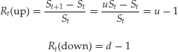
Real probabilities of states are typically constructed from the probabilities of a movement up or down. Call p the probability of a movement up; 1 −p is thus the probability of a movement down. Suppose that the state s, which is identified by a price path, has k movements up and T−k movements down. The probability of the state s is

Consider the final date T. Each of the possible flnal prices can be obtained through

paths with k movements up and T − k movements down. The probability distribution of final prices is therefore a binomial distribution:

Following the same reasoning, one can demonstrate that at any intermediate date the probability distribution of prices is a binomial distribution as follows:

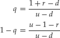
Next introduce a risk-free security. In the setting of a binomial model, a risk-free security is simply a security such that d = u = 1+r where r>0 is the positive risk-free rate. To avoid arbitrage it is clearly necessary that d<1+r<u. In fact, if the interest rate is inferior to both the up and down returns, one can make a sure profit by buying the risky asset and shorting the risk-free asset. If the interest rate is superior to both the up and down returns, one can make a sure profit by shorting the risky asset and buying the risk-free asset. Denote by bt the price of the risk-free asset at time t. From the definition of price movement in the binomial model we can write: bt = (1+r)tb0.

Risk-Neutral Probabilities for the Binomial Model

Let’s now compute the risk-neutral probabilities. In the setting of binomial models, the computation of risk-neutral probabilities is simple. In fact we have to impose the condition:

which we can explicitly write as follows:

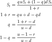
As we have assumed 0<d<1+r<u, the condition 0<q<1 holds. Therefore we can state that the unique risk-neutral probabilities are

The binomial model is complete and arbitrage free.

Suppose that there is more than one risky asset, for example two risky assets, in addition to the risk-free asset. At each time step each risky asset can go either up or down. Therefore there are four possible joint movements at each time step: uu, ud, du, dd that we identify with the states 1,2,3,4. Four probabilities must be determined at each time step; four equations are therefore needed. Two equations are provided by the martingale conditions:

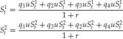
A third equation is provided by the fact that probabilities must sum to 1. The fourth condition, however, is missing. The model is incomplete.

The problem of approximating price processes when there are two stocks and one bond and where the stock prices follow two correlated lognormal processes has long been of interest to financial economists. As seen above, with two stocks and one bond available for trading, markets cannot be completed by dynamic trading. This is not the case in the continuous-time model, in which markets can be completed by continuous trading in the two stocks and the bond. Different solutions to this problem have been proposed in the literature.2

ARBITRAGE PRICING IN A DISCRETE-TIME, CONTINUOUS-STATE SETTING

Let’s now discuss the discrete-time, continuous-state setting. This is an important setting as it is, for example, the setting of the arbitrage pricing theory (APT) model.3

As in the previous discrete-time, discrete-state setting, we apply probabilistic concepts. The economy is represented by a probability space where Ω is the set of possible states, σ is the σ-algebra of events (formed, in this continuous-state setting, by a nondenumerable number of events), and P is a probability function. As the number of states is infinite, the probability of each state is zero and only events, in general, formed by nondenumerable states have a finite probability. There are only a finite number of dates from 0 to T. The propagation of information is represented by a finite filtration . In this case, the filtration is not equivalent to an information structure It.

Each security i is characterized by a payoff process dit and by a price process Sit. In this continuous-state setting, dit and Sit are formed by a finite number of continuous variables. As before, and are, respectively, the payoff and the price of the i-th asset at time and in state . All payoffs and prices are stochastic processes adapted to the filtration .

To develop an intuition for continuous-state arbitrage pricing, consider the previous multiperiod, finite-state case with a very large number M of states, M>>N where N is the number of securities. Recall from our earlier discussion that risk-neutral probabilities can be computed solving the following system of linear equations:

Recall also that at each date t the information structure It partitions the set of states into Mt subsets. Each partition therefore yields N× Mt equations and the system is formed by a total of

equation plus the probability normalizing equation. Consider that the previous system can be broken down, at each date t, into separate blocks formed by N equations (one for each asset) of the following type:

Each of these systems can be solved individually for the conditional probabilities . Recall that a system of this type admits a solution if and only if the coefficient matrix and the augmented coefficient matrix have the same rank. If the system is solvable, its solution will be unique if and only if the number of unknowns is equal to the rank of the coefficient matrix.

If the above system is not solvable, then there are arbitrage opportunities. This occurs if the payoffs of an asset are a linear combination of those of other assets, but its price is not the same linear combination of the prices of the other assets. This happens, in particular, if two assets have the same payoff in each state but different prices. In these cases, in fact, the rank of the coefficient matrix is inferior to the rank of the augmented matrix.

Under the assumption

this system, if it is solvable, will be undetermined. Therefore, there will be infinite equivalent risk-neutral probabilities and the market will not be complete. Going to the limit of an infinite number of states, the above reasoning proves, heuristically, that a discrete-time continuous-state market with a finite number of securities is inherently incomplete. In addition, there will be arbitrage opportunities only if the random variable that represents the payoff of an asset is a linear combination of the random variables that represent the payoffs of other assets, but the random variables that represent prices are not in the same relationship.

The above discussion can be illustrated in the case of multiple assets, each following a binomial model. If there are N linearly independent assets, the price paths in the interval (0, T) will form a total of states. In a binomial model, we can limit our considerations to one time step as the other steps are identical. In one step, each price Sit at time t can go up to Situi or down to Sitdi at time t+1. Given the prices at time t, there will be at the next time step, 2N possible combinations or di.

Suppose that there are 2N states and that each combination of prices identifies a state. This means that at each date t the information structure It partitions the set of states into 2Nt subsets. Each set of the partition is partitioned into 2N subsets at the next time step. This yields 2N(t+1) subsets at time t+1.

Note that this partitioning is compatible with any correlation structure between the random variables that represent prices. In fact, correlations depend on the value of the probability assigned to each state while the partitioning we assume depends on how different prices are assigned to different states.

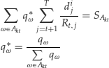
Risk-neutral probabilities can be determined solving the following system of martingale conditions:

which becomes, after dividing each equation by Sit, the following:

where wi(j) = ui or di for asset i in state j.

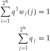
It can be verified that, under the previous assumptions and provided prices are positive, the above system admits infinite solutions. In fact, as N+1<2N, the number of equations is larger than the number of unknowns. Therefore, if the system is solvable it admits infinite solutions. To verify that the system is indeed solvable, let’s choose the first asset and partition the set of states into two events corresponding to the movement up or down of the same asset. Assign to these events probabilities as in the binomial model

Choose a second asset and partition each of the previous events into two events corresponding to the movements up or down of the second asset. We can now assign the following probabilities to each of the following four events:

It can be verified that these numbers sum to one. The same process can be repeated for each additional asset. We obtain a set of positive numbers that sum to one and that satisfy the system by construction. There are infinite other possible constructions. In fact, at each step, we could multiply probabilities by “correlation factors” (i.e., numbers that form a 2× 2 correlation matrix) and still obtain solutions to the system.

We can therefore conclude that a system of positive binomial prices such as the one above plus a risk-free asset is arbitrage-free and forms an incomplete market. If we let the number of states tend to infinity, the binomial distribution converges to a normal distribution. We have therefore demonstrated heuristically that a multivariate normal distribution plus a risk-free asset forms an incomplete and arbitrage-free market. Note that the presence of correlations does not change this conclusion.

Let’s now see under what conditions this conclusion can be changed. Go back to the multiple binomial model, assuming, as before, that there are N assets and T time steps. There is no logical reason to impose that the number of states be 2Nt. As we can consider each time step separately, suppose that there is only one time step and that there are a number of states less than or equal to the number of assets plus 1: . In this case, the martingale condition that determines risk-neutral probabilities becomes:

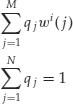
There are M equations and N+1 unknowns with . This system will either determine unique risk-neutral probabilities or will be unsolvable. Therefore, the market will be either complete and arbitrage-free or will exhibit arbitrage opportunities. Note that in this case we cannot use the constructive procedure used in the previous case.

What is the economic meaning of the condition that the number of states be less than or equal to the number of assets? To illustrate this point, assume that the number of states is . This means that we can choose K assets whose independent price processes identify all the states as in the previous case. Now add one more asset. This asset will go up or down not in specific states but in events formed by a number of states. Suppose it goes up in the event A and goes down in the event B. These events are determined by the value of the first K assets. In other words, the new asset will be a function of the first K assets. An interesting case is when the new asset can be expressed as a linear function of the first K assets. We can then say that the first K assets are factors and that any other asset is expressed as a linear combination of the factors.

Consider that, given the first K assets, it is possible to determine state-price deflators. These state-price deflators will not be uniquely determined. Any other price process must be expressed as a linear combination of state-price deflators to avoid arbitrage. If all price processes are arbitrage-free, the market will be complete if it is possible to determine uniquely the risk-neutral probabilities.

If we let the number of states become very large, the number of assets must become large as well. Therefore it is not easy to develop simple heuristic arguments in the limit of a large economy. What we can say is that in a large discrete economy where the number of states is less than or equal to the number of assets, if there are no arbitrage opportunities the market might be complete. If the market is complete and arbitrage-free, there will be a number of factors while all other processes will be linear combinations of these factors.

KEY POINTS

• The law of one price states that a given asset must have the same price regardless of the means by which one goes about creating that asset.
• Arbitrage is the simultaneous buying and selling of an asset at two different prices in two different markets.
• A finite-state one-period market is represented by a vector of prices and a matrix of payoffs.
• A state-price vector is a strictly positive vector such that prices are the product of the state-price vector and the payoff matrix.
• There is no arbitrage if and only if there is a state-price vector.
• A market is complete if an arbitrary payoff can be replicated by a portfolio.
• A finite-state one-period market is complete if there are as many linearly independent assets as states.
• A multiperiod finite-state economy is represented by a probability space plus an information structure.
• In a multiperiod finite-state market each security is represented by a payoff process and a price process.
• An arbitrage is a trading strategy whose payoff process is nonnegative and not always zero.
• A market is complete if any nonnegative payoff process can be replicated with a trading strategy.
• A state-price deflator is a strictly positive process such that prices are random variables equal to the conditional expectation of discounted payoffs.
• A martingale is a process such that at any time t its conditional expectation at time s, s>t coincides with its present value.
• In the absence of arbitrage there is an artificial probability measure in which all price processes, appropriately discounted, become martingales.
• Given a probability measure P, the probability measure Q is said to be equivalent to P if both assign probability zero to the same events.
• The binomial model assumes that there are two positive numbers, d and u, such that 0<d<u and such that at each time step the price S of the risky asset changes to dS or to uS.
• The distribution of prices of a binomial model is a binomial distribution.
• The binomial model is complete.

NOTES

1. The binomial model was first suggested for the pricing of options by Cox, Ross, and Rubinstein (1979), Rendleman and Bartter (1979), and Sharpe (1978).

2. See He (1990).

3. For an application of the principles discussed here to the APT, see Focardi and Fabozzi (2004).

REFERENCES

Cox, J. C., Ross, S. A., and Rubinstein, M. (1979). Option pricing: A simplified approach. Journal of Financial Economics 7:229–263.

Focardi, S. M., and Fabozzi, F. J. (2004). The Mathematics of Financial Modeling and Investment Management. Hoboken, NJ: John Wiley & Sons.

He, H. (1990). Convergence from discrete- to continuous-time contingent claims prices. Review of Financial Studies 3:523–546.

Rendleman, R. J., Jr., and Bartter, B. J. (1979). Two-state option pricing. Journal of Finance 24:1093–1110.

Sharpe, W. F. (1978). Investments. Englewood Cliffs, NJ: Prentice Hall.

Shleifer, A., and Vishny, R. W. (1997). The limits of arbitrage. Journal of Finance 52:35–55.