Quantitative Models to Value Convertible Bonds
Convertibles are ideal securities for arbitrage, because the convertible itself, namely the underlying stock and the associated derivatives, are traded along predictable ratios, and any discrepancy or misprice would give rise to arbitrage opportunities for fund managers. Traders use quantitative models to identify convertible bonds whose market value differs from their theoretical price. However, unlike callable bonds or putable bonds that have interest rate–embedded options, a convertible bond also has an embedded equity option. This complicates the quantitative modeling of these securities.
Quantitative models, or valuation models, for convertible bonds are divided into two categories: analytical models and numerical models. In this entry, we describe the more commonly used model in both of these categories.
ANALYTICAL MODELS
Ingersoll (1977) proposed a valuation model for convertible bonds based on the option theory and on the Black-Scholes option pricing model. The model’s main assumptions are:
- Markets operate continuously.
- There are no transaction costs.
- Share prices follow an Ito diffusion process.
- Securities prices have a lognormal distribution.
- The underlying stock volatility is constant.
Ingersoll’s model assumes that prices vary continuously, that is, there is always liquidity in the market and there are no limits to securities lending and short selling. It also assumes that the company’s market value follows an Ito diffusion process, that is, a continuous Brownian motion. Under this assumption, it is possible to set up a closed analytical formula to calculate the value of a convertible bond.
The model can be applied only to European convertibles, namely, convertibles that can be exercised only upon expiration. Moreover, the model makes it clear how complex the valuation of convertible bonds is, and it provides a highly interesting theoretical reference, in that it can reach an analytical solution to the valuation of convertibles. Yet, we know all too well that interest rates, credit spreads, currencies, and dividends are not constant, and the clauses and provisions written in the prospectus of a convertible are often highly varied and complicated, making it fairly difficult to apply analytical valuation models. This is why it is necessary to turn to numerical approximation models.
The Ingersoll Model
As just noted, the Ingersoll model provides an analytic solution for the pricing of a convertible bond, given some general market assumptions. The strongest assumptions are:
- Capital markets are perfect with no transaction costs, no taxes, and equal access to information for all investors.
- Trading takes place continuously in time and there are no restrictions against borrowing or short sales.
- The market value of the company follows an Ito diffusion process.
The Black-Scholes option pricing model is used to value the convertible bond as a contingent claim on the firm as a whole.
Consider a convertible bond that is convertible only at maturity, therefore with a European call option embedded. Let
![]()
equal the dilution factor, indicating the fraction of the common equity that would be held by the convertible bond issue’s owners if the entire issue were converted:
V = market value of the company
τ = maturity of the convertible bond
B = balloon payment (nominal value of the convertible bond)
r = interest rate
In light of the continuous-time analysis, the functional form to assume for the call price of a convertible bond is the exponential:
![]()
where
ρ = rate of change in the call price
σ2 = the instantaneous variance of returns of the stock underlying the convertible bond

is the cumulative normal distribution


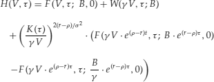
The value of the convertible bond is

To illustrate the model, let’s plot the function H with the following parameters:
B = 100
ρ = 0,02
γ = 0,2
σ2 = 5%
r = 7%
V ranges from 0 to 625.
The plots are shown in Figure 1. The straight lines cross at
Figure 1 Plot of a Convertible Bond Function for Different Firm Values

![]()
NUMERICAL MODELS
The most widely used mathematical models among hedge fund managers for the valuation of convertible bonds are numerical methods, among which are the binomial and trinomial trees, the three-dimensional binomial model, implied trees, and the Monte Carlo simulation model.
The binomial tree model was introduced by Cox, Ross, and Rubinstein (1979) and by Sharpe in his textbook (Sharpe, 1978). This model allows one to build a tree of possible share prices between now and the convertible’s maturity date. This tree is then used to find the convertible’s current value by calculating its value along all the tree’s nodes. In the binomial tree model, the tree has two branches that develop from every node, while in the trinomial tree model there are three branches diverging from each node. The higher the number of nodes, the more accurate the model is. The binomial model makes it possible to also value an American option that would otherwise find no solution in a closed form. If the number of time steps grows bigger, the binomial tree tends toward the Black-Scholes continuous formula for European options.
All these models are helpful when making a decision, but many of the options embedded in a convertible do not fit the models and therefore the fund manager’s skill and a rigorous risk management discipline become more precious. The manager’s art lies in finding innovative ways to evaluate convertible bonds without being swamped with too many details.
The trinomial tree model was introduced by Boyle (1986). The share price can move in three directions from every single node and therefore the number of time steps can be reduced to reach the same precision obtained with the binomial tree.
The Monte Carlo method, named after the casino of the Principality of Monaco, is a statistical simulation method, according to which data obtained through the generation of random numbers coming from a given statistical distribution is considered empirical and is used to estimate the parameters under consideration. Thousands of random samples are generated, derived from the assumed statistical distribution, which takes as parameters the maximum likelihood estimators using real data, and then these data are used to estimate the parameters under examination.
The Binomial Tree Model
Here, we will describe a version of the Cox-Ross-Rubinstein model as modified by Goldman Sachs. The binomial tree model can be used to evaluate convertible bonds with either an embedded European call option or an embedded American call option.
To determine the value of the convertible bond, it’s necessary to build four different trees in the following order:
In the first step we build the stock price tree. The binomial tree model allows us to build up a picture of how a stock is likely to perform between now and the maturity of the convertible bond (T). The number of nodes (N) is calculated from the maturity of the convertible bond according to the formula T · (T + 1)/2. The more nodes, the more accurate will be the model.
Between a node and the following node, the stock price can move upward or downward. The jump of the stock price depends on the length of the time interval Δt = T/N and on the stock price volatility σ. Therefore
![]()
The stock price, S, at each node is set equal to
![]()
where i = 0, 1, … , j
N is the time step and i is the number of upward moves.
The probability of a downward move in stock price at the next time step Δt is
![]()
while the probability of a downward move must be (1 − p), since the probability of going either up or down equals unity.
In the second step we build the conversion probability tree. We calculate the conversion probabilities backward, starting from the leaves of the stock price tree. If it’s optimal to convert the bond, the conversion probability is 1, otherwise it is 0. For the steps before the end of the tree, the conversion probability is 1 if it’s optimal to convert the bond; otherwise, it is equal to
![]()
In the third step we build the credit-adjusted spread tree. If the convertible bond is out-of-the-money, futures cash flows should be discounted to a rate equal to the risk-free rate, r, plus a credit spread, k, of that particular bond. In fact, if the stock price is much lower than the conversion price, the convertible bond behaves like a plain vanilla bond. If the convertible bond is in-the-money, future cash flows must be discounted at the risk-free rate. In this case, the convertible bond behaves like a stock. Therefore, instead of using a fixed discount rate r, in each node is calculated a discount rate rn,i and a conversion probability qn,i is used. The discount rate is equal to
![]()
In the fourth step, we build the convertible bond value tree. At each node of the tree, the price of the convertible bond is equal to the maximum between the conversion value of the bond and the face value plus the final coupon. The tree is built backward: from the leaves back to the root of the tree. The root of the tree is the price of the convertible bond.
If it’s optimal to convert the bond at a node, then that node is assigned the conversion value; otherwise, the price of the convertible bond is
![]()
where m is the conversion ratio.
For example, let’s determine the price of a convertible bond with the binomial tree method, starting with the following data:
T = 5 years (maturity)
Δt = 1 year (step)
N = 5 (number of nodes)
r = 4% (risk-free rate)
k = 2% (credit spread)
The convertible bond has nominal value 100 and coupon 10%.
m = 100% (conversion ratio)
S = 85 (stock price)
σ = 10% (stock volatility)
With the formulas discussed above we calculate
u = 1.1052 (upwards move)
d = 0.9048 (downwards move)
p = 0.6787 (probability of an upward move of the stock price in the next time interval Δt)
Figure 2 Binomial Trees Necessary to Determine the Value of a Convertible Bond

As shown in Figure 2 we built first the stock price tree, then the conversion probability tree, then the credit-adjusted spread tree, and finally the convertible bond value tree. The value in the root of the tree is 90.4, which is the price of the convertible bond.
KEY POINTS
- To implement strategies involving convertible bonds, traders and fund managers require a valuation model.
- Analytical models provide a closed-form solution for the value of a convertible bond, and the most commonly used model in practice is the Ingersoll model.
- While there are several models that fall into the realm of numerical models, the one commonly used is the binomial tree model, which requires the construction of a stock price tree, conversion probability tree, credit-adjusted spread tree, and convertible bond value tree that is calculated backward from the previous trees.
REFERENCES
Boyle, P. P. (1986). Option valuation using a three jump process. International Options Journal 3: 7–12.
Boyle, P. P. (1988). A lattice framework for option pricing with two state variables. Journal of Financial and Quantitative Analysis 23, 1: 1–12.
Black, F., and Scholes, M. (1973). The pricing of options and corporate liabilities. Journal of Political Economy 81, 3: 637–654.
Cox, J. C., Ross, S. A., and Rubinstein, M. (1979). Option pricing: A simplified approach. Journal of Financial Economics 7, 3: 229–263.
Cox, J. C. and Rubinstein, M. (1985). Option Markets. Englewood Cliffs, NJ: Prentice Hall.
Ingersoll, J. (1977). A contingent-claims valuation of convertible securities. Journal of Financial Economics 4, 2: 289–322.
Sharpe, W. F. (1978). Investments. Englewood Cliffs, NJ: Prentice Hall.
