
Mean-Variance Model for Portfolio Selection
The theory of portfolio selection presented in this entry, often referred to as mean-variance portfolio analysis or simply mean-variance analysis, is a normative theory. A normative theory is one that describes a standard or norm of behavior that investors should pursue in constructing a portfolio rather than a prediction concerning actual behavior.
Asset pricing theory goes on to formalize the relationship that should exist between asset returns and risk if investors behave in a hypothesized manner. In contrast to a normative theory, asset pricing theory is a positive theory—a theory that hypothesizes how investors behave rather than how investors should behave. Based on that hypothesized behavior of investors, a model that provides the expected return (a key input for constructing portfolios based on mean-variance analysis) is derived and is called an asset pricing model.
Together, portfolio selection theory and asset pricing theory provide a framework to specify and measure investment risk and to develop relationships between expected asset return and risk (and hence between risk and required return on an investment). However, it is critically important to understand that portfolio selection is a theory that is independent of any theories about asset pricing. The validity of portfolio selection theory does not rest on the validity of asset pricing theory.
It would not be an overstatement to say that modern portfolio theory has revolutionized the world of investment management. Allowing managers to quantify the investment risk and expected return of a portfolio has provided the scientific and objective complement to the subjective art of investment management. More importantly, whereas at one time the focus of portfolio management used to be the risk of individual assets, the theory of portfolio selection has shifted the focus to the risk of the entire portfolio. This theory shows that it is possible to combine risky assets and produce a portfolio whose expected return reflects its components, but with considerably lower risk. In other words, it is possible to construct a portfolio whose risk is smaller than the sum of all its individual parts!
Though practitioners realized that the risks of individual assets were related, before modern portfolio theory, they were unable to formalize how combining these assets into a portfolio impacted the risk at the entire portfolio level, or how the addition of a new asset would change the return–risk characteristics of the portfolio. This is because practitioners were unable to quantify the returns and risks of their investments. Furthermore, in the context of the entire portfolio, they were also unable to formalize the interaction of the returns and risks across asset classes and individual assets. The failure to quantify these important measures and formalize these important relationships made the goal of constructing an optimal portfolio highly subjective and provided no insight into the return investors could expect and the risk they were undertaking. The other drawback before the advent of the theory of portfolio selection and asset pricing theory was that there was no measurement tool available to investors for judging the performance of their investment managers.
SOME BASIC CONCEPTS
Portfolio theory draws on concepts from two fields: financial economic theory and probability and statistical theory. This section presents the concepts from financial economic theory used in portfolio theory. While many of the concepts presented here have a more technical or rigorous definition, the purpose is to keep the explanations simple and intuitive so that the importance and contribution of these concepts to the development of modern portfolio theory can be appreciated.
Utility Function and Indifference Curves
There are many situations where entities (i.e., individuals and firms) face two or more choices. The economic “theory of choice” uses the concept of a utility function to describe the way entities make decisions when faced with a set of choices. A utility function assigns a (numeric) value to all possible choices faced by the entity. The higher the value of a particular choice, the greater the utility derived from that choice. The choice that is selected is the one that results in the maximum utility given a set of constraints faced by the entity.
In portfolio theory too, entities are faced with a set of choices. Different portfolios have different levels of expected return and risk. Typically, the higher the level of expected return, the larger the risk. Entities are faced with the decision of choosing a portfolio from the set of all possible risk–return combinations, where when they like return, they dislike risk. Therefore, entities obtain different levels of utility from different risk–return combinations. The utility obtained from any possible risk–return combination is expressed by the utility function. Put simply, the utility function expresses the preferences of entities over perceived risk and expected return combinations.
A utility function can be expressed in graphical form by a set of indifference curves. Figure 1 shows indifference curves labeled u1, u2, and u3. By convention, the horizontal axis measures risk and the vertical axis measures expected return. Each curve represents a set of portfolios with different combinations of risk and return. All the points on a given indifference curve indicate combinations of risk and expected return that will give the same level of utility to a given investor. For example, on utility curve u1, there are two points u and u′, with u having a higher expected return than u′, but also having a higher risk. Because the two points lie on the same indifference curve, the investor has an equal preference for (or is indifferent to) the two points, or, for that matter, any point on the curve. The (positive) slope of an indifference curve reflects the fact that, to obtain the same level of utility, the investor requires a higher expected return in order to accept higher risk.
Figure 1 Indifference Curves
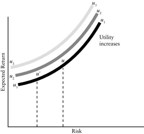
For the three indifference curves shown in Figure 1, the utility the investor receives is greater the further the indifference curve is from the horizontal axis because that curve represents a higher level of return at every level of risk. Thus, for the three indifference curves shown in the figure, u3 has the highest utility and u1 the lowest.
The Set of Efficient Portfolios and the Optimal Portfolio
Portfolios that provide the largest possible expected return for given levels of risk are called efficient portfolios. To construct an efficient portfolio, it is necessary to make some assumption about how investors behave when making investment decisions. One reasonable assumption is that investors are risk averse. A risk-averse investor is an investor who, when faced with choosing between two investments with the same expected return but two different risks, prefers the one with the lower risk.
In selecting portfolios, an investor seeks to maximize the expected portfolio return given his tolerance for risk. (Alternatively stated, an investor seeks to minimize the risk that he is exposed to given some target expected return.) Given a choice from the set of efficient portfolios, an optimal portfolio is the one that is most preferred by the investor.
Risky Assets vs. Risk-Free Assets
A risky asset is one for which the return that will be realized in the future is uncertain. For example, an investor who purchases the stock of Pfizer Corporation today with the intention of holding it for some finite time does not know what return will be realized at the end of the holding period. The return will depend on the price of Pfizer’s stock at the time of sale and on the dividends that the company pays during the holding period. Thus, Pfizer stock, and indeed the stock of all companies, is a risky asset.
Securities issued by the U.S. government are also risky. For example, an investor who purchases a U.S. government bond that matures in 30 years does not know the return that will be realized if this bond is held for only one year. This is because changes in interest rates in that year will affect the price of the bond one year from now and that will impact the return on the bond over that year.
There are assets, however, for which the return that will be realized in the future is known with certainty today. Such assets are referred to as risk-free or riskless assets. The risk-free asset is commonly defined as a short-term obligation of the U.S. government. For example, if an investor buys a U.S. government security that matures in one year and plans to hold that security for one year, then there is no uncertainty about the return that will be realized. The investor knows that in one year, the maturity date of the security, the government will pay a specific amount to retire the debt. Notice how this situation differs for the U.S. government security that matures in 30 years. While the 1-year and the 30-year securities are obligations of the U.S. government, the former matures in one year so that there is no uncertainty about the return that will be realized. In contrast, while the investor knows what the government will pay at the end of 30 years for the 30-year bond, he does not know what the price of the bond will be one year from now.
MEASURING A PORTFOLIO’S EXPECTED RETURN
We are now ready to define the actual and expected return of a risky asset and a portfolio of risky assets.
Measuring Single-Period Portfolio Return
The actual return on a portfolio of assets over some specific time period is straightforward to calculate using the formula:
where
Rp = rate of return on the portfolio over the period
Rg
= rate of return on asset g over the period
wg
= weight of asset g in the portfolio (i.e., market value of asset g as a proportion of the market value of the total portfolio) at the beginning of the period
G
= number of assets in the portfolio
In shorthand notation, equation (1) can be expressed as follows:
Equation (2) states that the return on a portfolio (Rp) of G assets is equal to the sum over all individual assets’ weights in the portfolio times their respective return. The portfolio return Rp is sometimes called the holding period return or the ex post return.
For example, consider the following portfolio consisting of three assets:
| Asset | Market Value at the Beginning of Holding Period | Rate of Return over Holding Period |
| 1 | $6 million | 12% |
| 2 | $8 million | 10% |
| 3 | $11 million | 5% |
The portfolio’s total market value at the beginning of the holding period is $25 million. Therefore,
| w1 = $6 million/$25 million = 0.24, or 24% and R1 = 12% |
| w2 = $8 million/$25 million = 0.32, or 32% and R2 = 10% |
| w3 = $11 million/$25 million = 0.44, or 44% and R3 = 5% |
Notice that the sum of the weights is equal to 1. Substituting into equation (1), we get the holding period portfolio return,
![]()
The Expected Return of a Portfolio of Risky Assets
Equation (1) shows how to calculate the actual return of a portfolio over some specific time period. In portfolio management, the investor also wants to know the expected (or anticipated) return from a portfolio of risky assets. The expected portfolio return is the weighted average of the expected return of each asset in the portfolio. The weight assigned to the expected return of each asset is the percentage of the market value of the asset to the total market value of the portfolio. That is,
(3) ![]()
The E() signifies expectations, and E(RP) is sometimes called the ex ante return, or the expected portfolio return over some specific time period.
The expected return, E(Ri), on a risky asset i is calculated as follows. First, a probability distribution for the possible rates of return that can be realized must be specified. A probability distribution is a function that assigns a probability of occurrence to all possible outcomes for a random variable. Given the probability distribution, the expected value of a random variable is simply the weighted average of the possible outcomes, where the weight is the probability associated with the possible outcome.
In our case, the random variable is the uncertain return of asset i. Having specified a probability distribution for the possible rates of return, the expected value of the rate of return for asset i is the weighted average of the possible outcomes. Finally, rather than use the term “expected value of the return of an asset,” we simply use the term “expected return.” Mathematically, the expected return of asset i is expressed as
where
Rn
= the nth possible rate of return for asset i
pn
= the probability of attaining the rate of return Rn for asset i
N
= the number of possible outcomes for the rate of return
How do we specify the probability distribution of returns for an asset? We shall see later on in this entry that in most cases the probability distribution of returns is based on long-run historical returns. If there is no reason to believe that future long-run returns should differ significantly from historical long-run returns, then probabilities assigned to different return outcomes based on the historical long-run performance of an uncertain investment could be a reasonable estimate for the probability distribution. However, for the purpose of illustration, assume that an investor is considering an investment, stock XYZ, which has a probability distribution for the rate of return for some time period as given in Table 1. The stock has five possible rates of return and the probability distribution specifies the likelihood of occurrence (in a probabilistic sense) of each of the possible outcomes.
Table 1 Probability Distribution for the Rate of Return for Stock XYZ
| n | Rate of Return | Probability of Occurrence |
| 1 | 12% | 0.18 |
| 2 | 10% | 0.24 |
| 3 | 8% | 0.29 |
| 4 | 4% | 0.16 |
| 5 | −4% | 0.13 |
| Total | 1.00 |
Substituting into equation (4) we get
Thus, 7% is the expected return or mean of the probability distribution for the rate of return on stock XYZ.
MEASURING PORTFOLIO RISK
Investors have used a variety of definitions to describe risk. Markowitz (1952, 1959) quantified the concept of risk using the well-known statistical measure: the standard deviation and the variance. The former is the intuitive concept. For most probability density functions, about 95% of the outcomes fall in the range defined by two standard deviations above and below the mean. Variance is defined as the square of the standard deviation. Computations are simplest in terms of variance. Therefore, it is convenient to compute the variance of a portfolio and then take its square root to obtain standard deviation.
Variance and Standard Deviation as a Measure of Risk
The variance of a random variable is a measure of the dispersion or variability of the possible outcomes around the expected value (mean). In the case of an asset’s return, the variance is a measure of the dispersion of the possible rate of return outcomes around the expected return.
The equation for the variance of the expected return for asset i, denoted var(Ri), is
![]()
or
Using the probability distribution of the return for stock XYZ, we can illustrate the calculation of the variance:

The variance associated with a distribution of returns measures the tightness with which the distribution is clustered around the mean or expected return. Markowitz argued that this tightness or variance is equivalent to the uncertainty or riskiness of the investment. If an asset is riskless, it has an expected return dispersion of zero. In other words, the return (which is also the expected return in this case) is certain, or guaranteed.
Since the variance is squared units, as we know from earlier in this section, it is common to see the variance converted to the standard deviation by taking the positive square root:
![]()
For stock XYZ, then, the standard deviation is
![]()
The variance and standard deviation are conceptually equivalent; that is, the larger the variance or standard deviation, the greater the investment risk. (A criticism of the variance or standard deviation as a measure is discussed later in this entry.)
Measuring the Portfolio Risk of a Two-Asset Portfolio
Equation (5) gives the variance for an individual asset’s return. The variance of a portfolio consisting of two assets is a little more difficult to calculate. It depends not only on the variance of the two assets, but also upon how closely the returns of one asset track those of the other asset. The formula is
where
cov(Ri, Rj) = covariance between the return for assets i and j
In words, equation (6) states that the variance of the portfolio return is the sum of the squared weighted variances of the two assets plus two times the weighted covariance between the two assets. We will see that this equation can be generalized to the case where there are more than two assets in the portfolio.
Table 2 Probability Distribution for the Rate of Return for Asset XYZ and Asset ABC

Covariance
The covariance has a precise mathematical translation. Its practical meaning is the degree to which the returns of two assets covary or change together. The covariance is not expressed in a particular unit, such as dollars or percent. A positive covariance means the returns on two assets tend to move or change in the same direction, while a negative covariance means the returns tend to move in opposite directions. The covariance between any two assets i and j is computed using the following formula:
where
rin
= the nth possible rate of return for asset i
rjn
= the nth possible rate of return for asset j
pn
= the probability of attaining the rate of return rin and rjn for assets i and j
N
= the number of possible outcomes for the rate of return
To illustrate the calculation of the covariance between two assets, we use the two stocks in Table 2. The first is stock XYZ from Table 1 that we used earlier to illustrate the calculation of the expected return and the standard deviation. The other hypothetical stock is stock ABC, whose data are shown in Table 2. Substituting the data for the two stocks from Table 2 in equation (7), the covariance between stocks XYZ and ABC is calculated as follows:
Relationship between Covariance and Correlation
The correlation is related to the covariance between the expected returns for two assets. Specifically, the correlation between the returns for assets i and j is defined as the covariance of the two assets divided by the product of their standard deviations:
Dividing the covariance between the returns of two assets by the product of their standard deviations results in the correlation between the returns of the two assets. Because the correlation is a standardized number (i.e., it has been corrected for differences in the standard deviation of the returns), the correlation is comparable across different assets. The correlation between the returns for stock XYZ and stock ABC is
![]()
The correlation coefficient can have values ranging from +1.0, denoting perfect comovement in the same direction, to –1.0, denoting perfect comovement in the opposite direction. Also note that because the standard deviations are always positive, the correlation can only be negative if the covariance is a negative number. A correlation of zero implies that the returns are uncorrelated.
Measuring the Risk of a Portfolio Consisting of More than Two Assets
So far we have defined the risk of a portfolio consisting of two assets. The extension to three assets—i, j, and k—is as follows:

In words, equation (9) states that the variance of the portfolio return is the sum of the squared weighted variances of the individual assets plus two times the sum of the weighted pairwise covariances of the assets. In general, for a portfolio with G assets, the portfolio variance is given by
(10) 
PORTFOLIO DIVERSIFICATION
Often, one hears investors talking about diversifying their portfolio. By this an investor means constructing a portfolio in such a way as to reduce portfolio risk without sacrificing return. This is certainly a goal that investors should seek. However, the question is how to do this in practice.
Some investors would say that including assets across all asset classes could diversify a portfolio. For example, a investor might argue that a portfolio should be diversified by investing in stocks, bonds, and real estate. While that might be reasonable, two questions must be addressed in order to construct a diversified portfolio. First, how much should be invested in each asset class? Should 40% of the portfolio be in stocks, 50% in bonds, and 10% in real estate, or is some other allocation more appropriate? Second, given the allocation, which specific stocks, bonds, and real estate should the investor select?
Some investors who focus only on one asset class such as common stock argue that such portfolios should also be diversified. By this they mean that an investor should not place all funds in the stock of one corporation, but rather should include stocks of many corporations. Here, too, several questions must be answered in order to construct a diversified portfolio. First, which corporations should be represented in the portfolio? Second, how much of the portfolio should be allocated to the stocks of each corporation?
Prior to the development of portfolio theory, while investors often talked about diversification in these general terms, they did not possess the analytical tools by which to answer the questions posed above. For example, in 1945, Leavens (1945, p. 473) wrote:
An examination of some fifty books and articles on investment that have appeared during the last quarter of a century shows that most of them refer to the desirability of diversification. The majority, however, discuss it in general terms and do not clearly indicate why it is desirable.
Leavens illustrated the benefits of diversification on the assumption that risks are independent. However, in the last paragraph of his article, he cautioned:
The assumption, mentioned earlier, that each security is acted upon by independent causes, is important, although it cannot always be fully met in practice. Diversification among companies in one industry cannot protect against unfavorable factors that may affect the whole industry; additional diversification among industries is needed for that purpose. Nor can diversification among industries protect against cyclical factors that may depress all industries at the same time.
A major contribution of the theory of portfolio selection is that using the concepts discussed above, a quantitative measure of the diversification of a portfolio is possible, and it is this measure that can be used to achieve the maximum diversification benefits.
The Markowitz diversification strategy is primarily concerned with the degree of covariance between asset returns in a portfolio. Indeed a key contribution of Markowitz diversification is the formulation of an asset’s risk in terms of a portfolio of assets, rather than in isolation. Markowitz diversification seeks to combine assets in a portfolio with returns that are less than perfectly positively correlated, in an effort to lower portfolio risk (variance) without sacrificing return. It is the concern for maintaining return while lowering risk through an analysis of the covariance between asset returns that separates Markowitz diversification from a naive approach to diversification and makes it more effective.
Markowitz diversification and the importance of asset correlations can be illustrated with a simple two-asset portfolio example. To do this, we first show the general relationship between the risk of a two-asset portfolio and the correlation of returns of the component assets. Then we look at the effects on portfolio risk of combining assets with different correlations.
Portfolio Risk and Correlation
In our two-asset portfolio, assume that asset C and asset D are available with expected returns and standard deviations as shown:
| Asset | E(R) | SD(R) |
| Asset C | 12% | 30% |
| Asset D | 18% | 40% |
If an equal 50% weighting is assigned to both stocks C and D, the expected portfolio return can be calculated as shown:
![]()
The variance of the return on the two-stock portfolio from equation (6), using decimal form rather than percentage form for the standard deviation inputs, is

From equation (8),
![]()
so
![]()
Since SD(RC) = 0.30 and SD(RD) = 0.40, then
![]()
Substituting into the expression for var(Rp), we get
![]()
Taking the square root of the variance gives
The Effect of the Correlation of Asset Returns on Portfolio Risk
How would the risk change for our two-asset portfolio with different correlations between the returns of the component stocks? Let’s consider the following three cases for cor(RC, RD): +1.0, 0, and –1.0. Substituting into equation (11) for these three cases of cor(RC, RD), we get:
| cor(RC,RD) | E(Rp) | SD(Rp) |
| +1.0 | 15% | 35% |
| 0.0 | 15% | 25% |
| −1.0 | 15% | 5% |
As the correlation between the expected returns on stocks C and D decreases from +1.0 to 0.0 to –1.0, the standard deviation of the expected portfolio return also decreases from 35% to 5%. However, the expected portfolio return remains 15% for each case.
Table 3 Portfolio Expected Returns and Standard Deviations for Five Mixes of Assets C and D
Asset C: E(RC) = 12%, SD(RC) = 30%
Asset D: E(RD) = 18%, and SD(RD) = 40%
Correlation between Assets C and D = cor(RC,RD) = –0.5

This example clearly illustrates the effect of Markowitz diversification. The principle of Markowitz diversification states that as the correlation (covariance) between the returns for assets that are combined in a portfolio decreases, so does the variance (hence the standard deviation) of the return for the portfolio.
The good news is that investors can maintain expected portfolio return and lower portfolio risk by combining assets with lower (and preferably negative) correlations. However, the bad news is that very few assets have small to negative correlations with other assets! The problem, then, becomes one of searching among large numbers of assets in an effort to discover the portfolio with the minimum risk at a given level of expected return or, equivalently, the highest expected return at a given level of risk.
The stage is now set for a discussion of efficient portfolios and their construction.
CHOOSING A PORTFOLIO OF RISKY ASSETS
Diversification in the manner suggested by Markowitz leads to the construction of portfolios that have the highest expected return for a given level of risk. Such portfolios are called efficient portfolios.
Constructing Efficient Portfolios
The technique of constructing efficient portfolios from large groups of stocks requires a massive number of calculations. In a portfolio of G securities, there are (G2 – G)/2 unique covariances to estimate. Hence, for a portfolio of just 50 securities, there are 1,225 covariances that must be calculated. For 100 securities, there are 4,950. Furthermore, in order to solve for the portfolio that minimizes risk for each level of return, a mathematical technique called quadratic programming must be used. A discussion of this technique is beyond the scope of this entry. However, it is possible to illustrate the general idea of the construction of efficient portfolios by referring again to the simple two-asset portfolio consisting of assets C and D.
Recall that for two assets, C and D, E(RC) = 12%, SD(RC) = 30%, E(RD) = 18%, and SD(RD) = 40%. We now further assume that cor(RC,RD) = –0.5. Table 3 presents the expected portfolio return and standard deviation for five different portfolios made up of varying proportions of C and D.
Feasible and Efficient Portfolios
A feasible portfolio is any portfolio that an investor can construct given the assets available. The five portfolios presented in Table 3 are all feasible portfolios. The collection of all feasible portfolios is called the feasible set of portfolios. With only two assets, the feasible set of portfolios is graphed as a curve, which represents those combinations of risk and expected return that are attainable by constructing portfolios from all possible combinations of the two assets.
Figure 2 presents the feasible set of portfolios for all combinations of assets C and D. As mentioned earlier, the portfolio mixes listed in Table 3 belong to this set and are shown by the points 1 through 5, respectively. Starting from 1 and proceeding to 5, asset C goes from 100% to 0%, while asset D goes from 0% to 100%—therefore, all possible combinations of C and D lie between portfolios 1 and 5, or on the curve labeled 1–5. In the case of two assets, any risk–return combination not lying on this curve is not attainable since there is no mix of assets C and D that will result in that risk–return combination. Consequently, the curve 1–5 can also be thought of as the feasible set.
Figure 2 Feasible and Efficient Portfolios for Assets C and D

In contrast to a feasible portfolio, an efficient portfolio is one that gives the highest expected return of all feasible portfolios with the same risk. An efficient portfolio is also said to be a mean-variance efficient portfolio. Thus, for each level of risk there is an efficient portfolio. The collection of all efficient portfolios is called the efficient set.
The efficient set for the feasible set presented in Figure 2 is differentiated by the bold curve section 3–5. Efficient portfolios are the combinations of assets C and D that result in the risk–return combinations on the bold section of the curve. These portfolios offer the highest expected return at a given level of risk. Notice that two of our five portfolio mixes—portfolio 1 with E(Rp) = 12% and SD(Rp) = 20% and portfolio 2 with E(Rp) = 13.5% and SD(Rp) = 19.5%—are not included in the efficient set. This is because there is at least one portfolio in the efficient set (for example, portfolio 3) that has a higher expected return and lower risk than both of them. We can also see that portfolio 4 has a higher expected return and lower risk than portfolio 1. In fact, the whole curve section 1–3 is not efficient. For any given risk–return combination on this curve section, there is a combination (on the curve section 3–5) that has the same risk and a higher return, or the same return and a lower risk, or both. In other words, for any portfolio that results in the return/risk combination on the curve section 1–3 (excluding portfolio 3), there exists a portfolio that dominates it by having the same return and lower risk, or the same risk and a higher return, or a lower risk and a higher return. For example, portfolio 4 dominates portfolio 1, and portfolio 3 dominates both portfolios 1 and 2.
Figure 3 shows the feasible and efficient sets when there are more than two assets. In this case, the feasible set is not a line, but an area. This is because, unlike the two-asset case, it is possible to create asset portfolios that result in risk–return combinations that not only result in combinations that lie on the curve I–II–III, but all combinations that lie in the shaded area. However, the efficient set is given by the curve II–III. It is easily seen that all the portfolios on the efficient set dominate the portfolios in the shaded area.
Figure 3 Feasible and Efficient Portfolios with More Than Two Assetsa
aThe picture is for illustrative purposes only. The actual shape of the feasible region depends on the returns and risks of the assets chosen and the correlation among them.
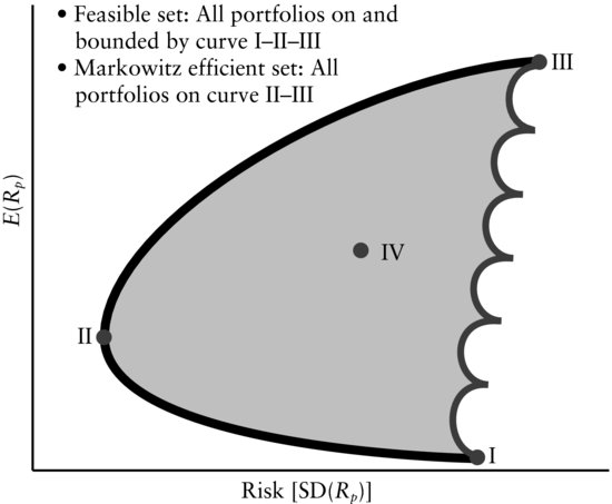
The efficient set of portfolios is sometimes called the efficient frontier because graphically all the efficient portfolios lie on the boundary of the set of feasible portfolios that have the maximum return for a given level of risk. Any risk–return combination above the efficient frontier cannot be achieved, while risk–return combinations of the portfolios that make up the efficient frontier dominate those that lie below the efficient frontier.
Choosing the Optimal Portfolio in the Efficient Set
Now that we have constructed the efficient set of portfolios, the next step is to determine the optimal portfolio.
Since all portfolios on the efficient frontier provide the greatest possible return at their level of risk, an investor or entity will want to hold one of the portfolios on the efficient frontier. Notice that the portfolios on the efficient frontier represent trade-offs in terms of risk and return. Moving from left to right on the efficient frontier, the risk increases, but so does the expected return. The question is which one of those portfolios should an investor hold? The best portfolio to hold of all those on the efficient frontier is the optimal portfolio.
Intuitively, the optimal portfolio should depend on the investor’s preference over different risk–return trade-offs. As explained earlier, this preference can be expressed in terms of a utility function.
In Figure 4, three indifference curves representing a utility function and the efficient frontier are drawn on the same diagram. An indifference curve indicates the combinations of risk and expected return that give the same level of utility. Moreover, the farther the indifference curve from the horizontal axis, the higher the utility.
Figure 4 Selection of the Optimal Portfolio

From Figure 4, it is possible to determine the optimal portfolio for the investor with the indi-fference curves shown. Remember that the investor wants to get to the highest indifference curve achievable given the efficient frontier. Given that requirement, the optimal portfolio is represented by the point where an indifference curve is tangent to the efficient frontier. In Figure 4, that is the portfolio PMEF*. For example, suppose that PMEF* corresponds to portfolio 4 in Figure 2. We know from Table 3 that this portfolio is made up of 25% of asset C and 75% of asset D, with an E(Rp) = 16.5% and SD(Rp) = 27.0%.
Table 4 Annualized Expected Returns, Standard Deviations, and Correlations between the Four Country Equity Indexes: Australia, Austria, Belgium, and Canada

Consequently, for the investor’s preferences over risk and return as determined by the shape of the indifference curves represented in Figure 4, and expectations for asset C and D inputs (returns and variance-covariance) represented in Table 3, portfolio 4 is the optimal portfolio because it maximizes the investor’s utility. If this investor had a different preference for expected risk and return, there would have been a different optimal portfolio.
At this point in our discussion, a natural question is how to estimate an investor’s utility function so that the indifference curves can be determined. Economists in the field of behavioral and experimental economics have conducted a vast amount of research in the area of utility functions. Though the assumption sounds reasonable that individuals should possess a function that maps the different preference choices they face, the research shows that it it not so straightforward to assign an individual with a specific utility function. This is because preferences may be dependent on circumstances, and those may change with time.
The inability to assign an investor with a specific utility function does not imply that the theory is irrelevant. Once the efficient frontier is constructed, it is possible for the investor to subjectively evaluate the trade-offs for the different return–risk outcomes and choose the efficient portfolio that is appropriate given his or her tolerance to risk.
Example Using the MSCI World Country Indexes
Now that we know how to calculate the optimal portfolios and the efficient frontier, let us take a look at a practical example. We start the example using only four assets and later show these results change as more assets are included. The four assets are the four country equity indexes in the MSCI World Index for Australia, Austria, Belgium, and Canada.
Let us assume that we are given the annualized expected returns, standard deviations, and correlations between these countries as presented in Table 4. The expected returns vary from 7.1% to 9%, whereas the standard deviations range from 16.5% to 19.5%. Furthermore, we observe that the four country indexes are not highly correlated with each other—the highest correlation, 0.47, is between Austria and Belgium. Therefore, we expect to see some benefits of portfolio diversification.
Figure 5 shows the efficient frontier for the four assets. We observe that the four assets, represented by the diamond-shaped marks, are all below the efficient frontier. This means that for a targeted expected portfolio return, the mean-variance portfolio has a lower standard deviation. A utility maximizing investor, measuring utility as the trade-off between expected return and standard deviation, will prefer a portfolio on the efficient frontier over any of the individual assets.
Figure 5 The Mean-Variance Efficient Frontier of Country Equity Indexes of Australia, Austria, Belgium, and Canada
Note: Constructed using the data in Table 4. The expected return and standard deviation combination of each country index is represented by a diamond-shaped mark. The global minimum variance portfolio (GMV) is represented by a solid circle. The portfolios on the curves above the GMV portfolio constitute the efficient frontier.

The portfolio at the leftmost end of the efficient frontier (marked with a solid circle in Figure 5) is the portfolio with the smallest obtainable standard deviation. It is called the global minimum variance (GMV) portfolio.
Increasing the Asset Universe
We know that by introducing more (low correlating) assets, for a targeted expected portfolio return, we should be able to decrease the standard deviation of the portfolio. In Table 5, the assumed annualized expected returns, standard deviations, and correlations of 18 countries in the MSCI World Index are presented.
Table 5 Annualized Expected Returns, Standard Deviations, and Correlations between 18 Countries in the MSCI World Index

Figure 6 illustrates how the efficient frontier moves outwards and upwards as we go from 4 to 12 assets and then to 18 assets. By increasing the number of investment opportunities, we increase the level of possible diversification thereby making it possible to generate a higher level of return at each level of risk.
Figure 6 The Efficient Frontier Widens as the Number of Low Correlated Assets Increase
Note: The efficient frontiers have been constructed with 4, 12, and 18 countries (from the innermost to the outermost frontier) from the MSCI World Index. The portfolios on the curves above the GMV portfolio constitute the efficient frontiers for the three cases.

Adding Short Selling Constraints
So far in this section, our theoretical derivations imposed no restrictions on the portfolio weights other than having them add up to one. In particular, we allowed the portfolio weights to take on both positive and negative values; that is, we did not restrict short selling. In practice, many portfolio managers cannot sell assets short. This could be for investment policy or legal reasons, or sometimes just because particular asset classes are difficult to sell short such real estate. In Figure 7, we see the effect of not allowing for short selling. Since we are restricting the opportunity set by constraining all the weights to be positive, the resulting efficient frontier is inside the unconstrained efficient frontier.
Figure 7 The Effect of Restricting Short Selling: Constrained versus Unconstrained Efficient Frontiers Constructed from 18 Countries from the MSCI World Index
Note: The portfolios on the curves above the GMV portfolio constitute the efficient frontiers.

ROBUST PORTFOLIO OPTIMIZATION
Despite the great influence and theoretical impact of modern portfolio theory, today full risk–return optimization at the asset level is primarily done only at the more quantitatively oriented asset management firms. The availability of quantitative tools is not the issue—today’s optimization technology is mature and much more user-friendly than it was at the time Markowitz first proposed the theory of portfolio selection—yet many asset managers avoid using the quantitative portfolio allocation framework altogether.
A major reason for the reluctance of portfolio managers to apply quantitative risk-return optimization is that they have observed that it may be unreliable in practice. Specifically, mean-variance optimization (or any measure of risk for that matter) is very sensitive to changes in the inputs (in the case of mean-variance optimization, such inputs include the expected return and variance of each asset and the asset covariance between each pair of assets). While it can be difficult to make accurate estimates of these inputs, estimation errors in the forecasts significantly impact the resulting portfolio weights. As a result, the optimal portfolios generated by the mean-variance analysis generally have extreme or counterintuitive weights for some assets.1 Such examples, however, are not necessarily a sign that the theory of portfolio selection is flawed; rather, that when used in practice, the mean-variance analysis as presented by Markowitz has to be modified in order to achieve reliability, stability, and robustness with respect to model and estimation errors.
It goes without saying that advances in the mathematical and physical sciences have had a major impact upon finance. In particular, mathematical areas such as probability theory, statistics, econometrics, operations research, and mathematical analysis have provided the necessary tools and discipline for the development of modern financial economics. Substantial advances in the areas of robust estimation and robust optimization were made during the 1990s, and have proven to be of great importance for the practical applicability and reliability of portfolio management and optimization.
Any statistical estimate is subject to error—that is, estimation error. A robust estimator is a statistical estimation technique that is less sensitive to outliers in the data and is not driven by one particular set of observations of the data. For example, in practice, it is undesirable that one or a few extreme returns have a large impact on the estimation of the average return of a stock. Nowadays, statistical techniques such as Bayesian analysis and robust statistics are more commonplace in asset management. Taking it one step further, practitioners are starting to incorporate the uncertainty introduced by estimation errors directly into the optimization process. This is very different from traditional mean-variance analysis, where one solves the portfolio optimization problem as a problem with deterministic inputs (i.e., inputs that are assumed to be known with certainty), without taking the estimation errors into account. In particular, the statistical precision of individual estimates is explicitly incorporated into the portfolio allocation process. Providing this benefit is the underlying goal of robust portfolio optimization.2
Modern robust optimization techniques allow a portfolio manager to solve the robust version of the portfolio optimization problem in about the same time as needed for the traditional mean-variance portfolio optimization problem. The robust approach explicitly uses the distribution from the estimation process to find a robust portfolio in a single optimization, thereby directly incorporating uncertainty about inputs in the optimization process. As a result, robust portfolios are less sensitive to estimation errors than other portfolios, and often perform better than optimal portfolios determined by traditional mean-variance portfolios. Moreover, the robust optimization framework offers greater flexibility and many new interesting applications. For instance, robust portfolio optimization can exploit the notion of statistically equivalent portfolios. This concept is important in large-scale portfolio management involving many complex constraints such as transaction costs, turnover, or market impact. Specifically, with robust optimization, a portfolio manager can find the best portfolio that (1) minimizes trading costs with respect to the current holdings and (2) has an expected portfolio return and variance that are statistically equivalent to those of the classical mean-variance portfolio.3
KEY POINTS
- Markowitz quantified the concept of diversification through the statistical notion of the covariances between individual securities that make up a portfolio and the overall standard deviation of the portfolio.
- A basic assumption behind modern portfolio theory is that an investor’s preferences over portfolios with different expected returns and variances can be represented by a function (utility function).
- The basic principle underlying modern portfolio theory is that for a given level of expected return an investor would choose the portfolio with the minimum variance from among the set of all possible portfolios.
- Minimum variance portfolios are called mean-variance efficient portfolios. The set of all mean-variance efficient portfolios is called the efficient frontier. The portfolio on the efficient frontier with the smallest variance is called the global minimum variance portfolio (GMVP).
- The efficient frontier moves outwards and upwards as the number of (not perfectly correlated) securities increases. The efficient frontier shrinks as constraints are imposed upon the portfolio.
- An advancement in the theory of portfolio selection is the development of estimation techniques that generate more robust mean-variance estimates along with optimization techniques that result in optimized portfolios being more robust to the mean-variance estimates used.
NOTES
1. See Best and Grauer (1991) and Chopra and Ziember (1993).
2. There are two approaches that have been suggested for dealing with this problem. One is the application of estimation by using a statistical technique known as Bayes analysis. (See Rachev, Hsu, Bagasheva, and Fabozzi, 2008.) The Black-Litterman model uses this approach. (See Black and Litterman, 1990.) The other approach is using a resampling methodology as suggested by Michaud (2001). A study by Markowitz and Usmen (2003) found that the resampled approach is superior to that of a Bayesian approach.
3. For a discussion of these models, see Fabozzi, Kolm, Pachamanova, and Focardi (2007).
REFERENCES
Best, M. J., and Grauer, R. R. (1991). On the sensitivity of mean-variance efficient portfolios to changes in asset means: Some analytical and computational results. Review of Financial Studies 4: 315–342.
Black, R., and Litterman, R. (1990). Asset allocation: Combining investor views with market equilibrium. Goldman, Sachs & Co., Fixed Income Research.
Chopra, V. K., and Ziemba, W. T. (1993). The effect of errors in means, variances, and covariances on optimal portfolio choice. Journal of Portfolio Management 19: 6–11.
Fabozzi, F. J., Kolm, P. N., Pachamanova, D., and Focardi, S. M. (2007). Robust Portfolio Optimization and Management. Hoboken, NJ: John Wiley & Sons.
Leavens, D. H. (1945). Diversification of investments. Trusts and Estates 80: 469–473.
Markowitz, H. M. (1952). Portfolio selection. Journal of Finance 7: 77–91.
Markowitz, H. M. (1959). Portfolio Selection: Efficient Diversification of Investments, Cowles Foundation Monograph 16. New York: John Wiley & Sons, 1959.
Markowitz, H. M., and Usmen, N. (2003). Diffuse priors vs. resampled frontiers: An experiment. Journal of Investment Management 1: 9–25.
Michaud, R. (2001). Efficient Asset Management: A Practical Guide to Stock Portfolio Optimization and Asset Allocation. New York: Oxford University Press.
Rachev, S. T., Hsu, J., Bagasheva, B., and Fabozzi, F. J. (2008). Bayesian Methods in Finance. Hoboken, NJ: John Wiley & Sons.