
The Concept and Measures of Interest Rate Volatility
In this entry, we introduce the concepts of market volatility and discuss how it is measured. The dynamics of rates are subject to market forces, mean reversion, and combinations of diffusions and jumps.
BASIC DEFINITIONS AND FIRST FINDINGS
We can't tell in advance what interest rates will be. Investors may be either enriched or bankrupted from sudden changes in interest rates. Financial institutions devote considerable resources to risk management and hedging. Yet, if future interest rates were deterministic, there would be no need to hedge. Coping with uncertainty is a central feature of investment markets.
The pricing of options and embedded-options instruments utilizes a statistical concept to describe the magnitude of potential interest rates changes. The key notion is the volatility of interest rates. While this term conjures up images of instability, flares of activity, and unpredict-ability, it is actually a very specific description of the range of possible outcomes. More precisely, volatility can be defined as the standard deviation of a rate's annualized daily increments. Table 1 provides an example for yields on the 10-year Treasury measured over 10 consecutive business days. As part of the measurement, we will be taking a daily time series and then transforming into “absolute returns” and “relative returns”—much like measuring portfolio performance.
Table 1 Example of Volatility Calculations

The absolute rate changes are computed by taking the difference between the interest rates on successive days. The relative changes are computed by dividing the absolute change by the starting rate. For example, for the first day the absolute change is 5.00343 − 5.03234 = −0.0289. The relative increment is −0.0289/5.03234 = −0.0057. In order to calculate the daily volatility, we just take the standard deviation of the daily absolute and relative change series. In the example above, the standard deviations are 0.048 (absolute increments) and 0.00966 (relative increments). The former number is the standard deviation for daily absolute increments; the latter number represents that of the daily relative changes. To compute volatility, we place these daily measures on an annual basis scaling by the number of trading days in the year (approximately 260):
Thus, in our example of the 10-day yield series, we would calculate the annual volatility as 77.3 basis points (absolute) or 15.57% (relative). The relative volatility times the average yield for the period 0.1557 × 4.983 = 0.776 is close to the absolute yield volatility of 0.773—as one would expect.
The second relevant clarification may damage a naïve understanding of volatility as the annual standard deviation. Volatility measures only the pace of uncertainty; this concept does not assume the daily-measured volatility remains constant over time, just as when driving in traffic with starts and stops there is a difference between instantaneous speed and the average velocity. Third, an important assumption for annualizing the daily volatilities is that the daily increments are serially independent. If there is a relationship between rate changes on one day and another day, then we say there is serial correlation. The “square-root rule” will not be an accurate measure of the annual volatility if there is serial correlation in the random process. Figure 1 illustrates that volatility has been volatile.
In the 1980s, both volatility measures exhibited instability, although the relative one appeared to be much more stable. However, since the 1990s, the absolute volatility measure has become more stable, oscillating around 1% (100 basis points). Based on these observations, it is not hard to understand why during different time periods, the relative volatility was moving inversely, and the absolute volatility directly, with respect to the rate level. Aside from the explicit level-related effect, both volatility measures seemingly synchronously react to economic disturbances. Pricing in the interest rate options market reflects these important findings.
Figure 1 History of Volatility for the 10-year Treasury Yield

Figure 2 Historical Volatility Term Structure for the Swap Rates
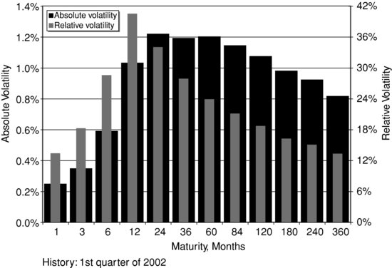
Different points of the yield curve have differing volatility, too. This observation suggests that not only do the rates have a “term structure,” but their volatility has a term structure as well. A hump shape of such a volatility curve is often observed (see Figure 2). It can be attributed to (1) absence of change in the short rates unless regulators take actions and (2) the dampening force of the mean reversion. We will explain both factors further in the entry.
A DIFFUSIVE MODEL FOR RANDOMNESS
Can we describe the randomness mathematically? It is perhaps simpler than it sounds. In fact, having become acquainted with volatility, we did most of the task. A general diffusive model for an interest rate process that describes how interest rates will vary over time, r(t), will have the following form:
What does this mean? Notations dr and dt refer to small increments measured over infinitesimally short time. Variable dz represents small changes in z(t) which is called Brownian motion, also known as the Wiener process. It is the source of randomness. We cannot control the exact value of this variable. Drift and volatility describe how the changes in rates are related to changes in time and the random variable dz. Mathematical model (1) can be thought of in the following way: The change in interest rate over a small time period is the result of a number representing systematic drift times the amount of time change plus a random shock scaled by the amount of volatility.
![]()
A Brief Excursion to Brownian Motion
Brownian motion:
- Is continuous
- Is normally distributed
- Has a zero mean (“centered”)
- Has time increments that are serially independent
- Has its own volatility scaled to 1
Therefore, z(t) has a standard deviation of ![]() (for the same reason that a square root appears in the annualization of daily volatility). Any particular function z(t) is said to be a “realization” or a “sample path” of the Brownian motion. The Brownian motion, therefore, can be thought of as a container of random paths subject to the conditions described above. Figure 3 depicts a sample path and the single- and double-standard deviation zones.
(for the same reason that a square root appears in the annualization of daily volatility). Any particular function z(t) is said to be a “realization” or a “sample path” of the Brownian motion. The Brownian motion, therefore, can be thought of as a container of random paths subject to the conditions described above. Figure 3 depicts a sample path and the single- and double-standard deviation zones.
With the use of volatility multiples, we can scale the rate process to any volatility level. The drift variable simulates a systematic, nonrandom tendency. For example, it can model a central tendency function known as mean reversion. Equation (1) is called the stochastic differential equation. Both multiples, drift and volatility do not have to be constants. They can be functions of time, t, and rate, r. Any particular specification of drift(t,r) and volatility(t,r) leads to a specific rate model, but not necessarily a good one. At this stage, it is enough to understand that a good model can be a strong quantitative pricing tool. Although we cannot know what the random variable z(t) is going to do, we, at least, can simulate its behavior with a large number of random scenarios. The Monte Carlo method draws on this idea. On the other hand, we may be able to do some intelligent analytical work making the brute-force simulations unnecessary. We could also make sure that the model is consistent with (“calibrated to”) prices of widely traded interest rate instruments; then we will feel more confident applying it to the exotic options or the market for mortgage-backed securities (MBSs) and asset-backed securities (ABSs).
Figure 3 Brownian Motion's Sample Path with Deviation Zones

MEAN REVERSION AND MARKET STABILITY
Consider the following special form of equation (1): dr = 5rdt + σdz. Can this equation model an actual interest rate? Since the formula shows that the change in interest rate increases with changes in time, the average rate will continue to grow. Utilizing calculus, we note that the solution to this equation will not only grow with time, but will grow exponentially as it contains an e5t term. Since interest rates cannot increase exponentially forever (at least, they never have), we need to dismiss this formula as inappropriate for the job.
How about dr = σdz? The drift is chosen to be zero, and provided that the initial value r(0) is known, the process will randomly evolve around this value, on average. Whether the initial rate is high or low, the model will stay centered around it. The standard deviation, as we already know, will grow as ![]() . This may not be a very good thing either. A century from now, the magnitude of the standard deviation will be huge, at ten times annual volatility. Figure 1B demonstrated that interest rates tend to stay within a range.
. This may not be a very good thing either. A century from now, the magnitude of the standard deviation will be huge, at ten times annual volatility. Figure 1B demonstrated that interest rates tend to stay within a range.
Both models briefly reviewed above suffer with the same disease: They are unstable. Observable objects in economy, finance, engineering, or physics tend to be stable; otherwise, they would not be able to exist long enough to be observed. The feature making financial markets stable is known as mean reversion. It is simply a properly chosen specification of the drift term that would ensure the dampening effect (also known as central tendency). If the rate randomly has grown too high or fallen too low, the drift term will help “return” it back. Here is an example:
where mean reversion parameter a > 0. This time, the solution will contain e−at, a decaying component that indicates stability. The mean converges to parameter r∞, the long-term equilibrium (now we see the point for this strange notation). The standard deviation will grow with time as
![]()
and converges to
![]()
as the horizon extends. Figure 4 compares the standard deviation (lines launching from the origin) and equivalent (“average”) volatility for different levels of mean reversion including the zero one (σ = 1% was assumed).
Figure 4 Standard Deviation and Average Volatility for Different Values of a
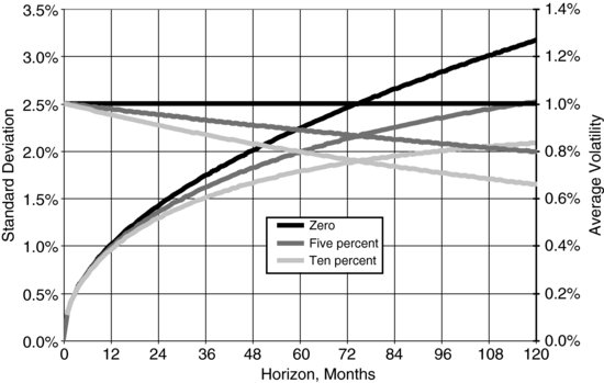
Mean reversion, therefore, stabilizes the market. It also explains why volatility is typically measured on a daily basis; in the presence of mean reversion, the average volatility measured over a time horizon generally depends on this horizon. For example, if a = 10%, only 95% of actual volatility is seen in annual increments.
If r(t) in (2) is the short market rate, then every other rate (the 5-year, the 10-year, etc.) can be derived as a function of it. In particular, for mean-reverting models, volatility of long rates should eventually fade with maturity of the rate, and it does happen as seen in Figure 2. Mathematically, it is a direct consequence of the mean reversion: The short rate's uncertainty gets limited going forward, thereby making long-term bonds less volatile now. Economically, discount rates for very remote cash flows should be almost certain; otherwise their present values would be infinitely risky.
Does it seem that model (2) makes sense? Well, Vasicek (1977) noticed it, as one of the first interest rate models. It is been popular and important since and was a basis for many of the models that are used today.
THE RATE DISTRIBUTION
Equation (2) is a linear stochastic differential equation disturbed by a Brownian motion. The math tells us that the output of this equation, rate r(t), is going to be normally distributed. Although it makes the model tractable, the negative rates are not precluded, which may or may not be a problem. Arguably, the actual rates should stay positive—at least, they almost always have been. When using process (2), odds of negative rates grow with future time, as the present value falls. In addition, mortgages and related securities are amortizing and may have small balances and cash flows years from now. Levin (2004) provided a quantitative support for the use of normal distribution by showing it does not distort options’ value materially.
Figure 5 Jumpy and Continuous Interest Rates

The fact that a Brownian motion is normally distributed does not require that the rate process be such. For example, considering exponential transformation R = exp(r) and using R as the rate, rather than r, we ensure that the rate remains positive. Such a process is said to have lognormal distribution. The mean and standard deviation for this known distribution is explicitly stated through the mean μ and the standard deviation σ of the original variable, r(t):

Another popular example is the squared transformation, R = r2, that also guarantees that rate R stays positive; the distribution of such defined rate is known as noncentral χ2. For the squared transformation,
![]()
INTEREST RATE JUMPS
Stochastic differential equation (1) is not the most general mathematical form of a random process. It applies only to diffusions, that is, continuous random processes. Stochastic calculus considers many other forms of randomness; an important one is called random jumps or random events. To appreciate this type of randomness, let us consider the history of three rates, the 1-month London Interbank Offered Rate (LIBOR) (“LIBOR 01”), the 2-year swap (“LIBOR 24”), and the 10-year swap rate (“LIBOR 120”), depicted in Figure 5.
Both swap rates change almost continuously, day after day, and little by little, at times randomly oscillating, in response to the market forces. The 1-month rate was changing in a suspiciously smooth fashion between sudden jumps featuring apparent and prolonged plateaus that are not seen for the swap rates. For example, in 2002 to 2004, it had been barely changing for a while, and then plunged responding to the Fed's actions. Furthermore, whereas the visual dynamics for all three rates seem to resemble one another, statistical measurements of correlation between daily increments overwhelmingly reject such a conclusion. For this 18-year-long history (over 4,500 observations) we computed a small 7% correlation between daily increments of the 1-month and the 2-year rates, and an even smaller 4% correlation between 1-month and 10-year rates. What if we measure correlations between increments in monthly averages (216 observations), thereby filtering out the disparity between daily dynamics? Then the 7% goes way up to 46% and the 4% to 24%, and the interrate correlations continue to improve steadily as we extend the averaging period (Table 2).
Table 2 Empirical Correlations between Periodic Increments, 1992–2010 History

These objective facts suggest that a stochastic diffusive model suitable for swap rates may be not perfectly appropriate for short rates. A random jump component may be necessary to explain the actual short-rate behavior and associated option pricing. One popular mathematical form of jumps is the Poisson process. It is simply a random occurrence of events described by a single parameter λ called frequency or intensity. The average number of events to occur during a time interval of t is equal to λt; curiously enough the variance of this number is equal to λt too. Probability that we will have exactly j events during this time interval is equal to e−λt(λt)j/j! It is only the period's length that really matters, not when the period starts—for this reason, the Poisson process can't be used to describe, say, human deaths or bulb failures when the attained age is a strong factor. However, it is plausible to assume that the Poisson jumps describe some events in financial markets.
Aside from the jumps’ arrival, the size of jumps can be also random. Merton (1976) introduced an option-pricing model when the underlying process includes Poisson jumps with normally distributed magnitude. Using mathematical notations, we can express the model as
where N is the Poisson-Merton jump variable. When jump occurs, dN is drawn from the standard normal distribution N[0,1]; it stays 0 otherwise. In a less strict notations,

The practical difference between random shock and random jump is that, for a small time interval, the former is small, but nonzero, whereas the latter is mostly zero and rarely finite. Hence, equation (3) describes a more general stochastic process combining diffusion and jumps (“jump-diffusion”). Notably, mathematical variance of the Poisson process N(t) is too proportional to the time horizon t. This fact allows aligning interpretations of σd ≡ Volatility and σj ≡ Jump Volatility: for very small t, the standard deviation of r(t) is equal to
![]()
meaning that the mixed volatility will be simply
![]()
Furthermore, if we generalize the linear mean-reverting Vasicek model given by (2) by adding a jump term, then expressions for the mean and the standard deviation of r(t) won't change; it will be enough to replace σ.
At first, it is tempting to interpret a jump-diffusion process as diffusion with another volatility scale. In reality, probability distributions of these two stochastic patterns are different. Inclusion of jumps “fattens” the distribution's tail (see Table 3) and is much more suitable for modeling and pricing rare events like a corporation's defaults or credit downgrade, a financial crisis, reaching a very remote option's strike, or change in the short rate over a fairly short horizon.
Table 3 Comparison of Distribution's Tails for Poisson-Merton Jump Processes

Models with Poisson-Merton processes converge to normal when the value of λt is large (frequent jumps are similar to diffusion), but may produce significantly different results when it is small.
Stochastic differential equations (1) and (3) can be viewed as building blocks for the interest rate modeling. Some models used today in the financial industry are multifactor with the short rate r(t) defined not as the solution to equations (1) or (3), but as their sum. When modeling LIBOR, neither the jump arrivals have to be Poissonian, nor the magnitude has to be normal. For example, Chan et al. (2003) developed a model with rate jumps timed to periodic Fed meetings, and the magnitude being a random multiple of 25 bps. There exist other modeling views at interest rate dynamics that we don't cover in this entry including continuous randomness with stochastic volatility levels; see James and Webber (2000) for a comprehensive overview.
KEY POINTS
- The most common way of simulating interest rates' uncertainty is employing stochastic differential equations containing drift and volatility terms.
- In older times, absolute volatility was directionally related to the rate's level; this relationship has gradually disappeared.
- The drift term must contain a mean reversion, that is, stabilization force.
- Actual short rates (LIBOR) have been historically jumpy and require adding random jumps to diffusions.
ACKNOWLEDGMENTS
The author wishes to thank Andrew Davidson for his help in shaping this material, Will Searle for his comments, and Nancy Davidson for her editorial work.
REFERENCES
Chan, Y.-K., Bhattacherjee, R., Russell, R., and Teytel, M. (2003). A New Term-Structure Model Based on Federal Funds Target. Citigroup, Mortgage Securities.
James, J. and Webber, N. (2000). Interest Rate Modeling: Financial Engineering. New York: John Wiley & Sons.
Levin, A. (2004). Interest rate model selection. Journal of Portfolio Management 30, 2: 74–86.
Levin, A. (2001). A tractable skew-and-smile model. The Dime Bancorp, Working Paper.
Merton, R. (1976). Option pricing when underlying stock returns are discontinuous. Journal of Financial Economics 3: 125–144.
Vasicek, O. (1977). An equilibrium characterization of the term structure. Journal of Financial Economics 5: 177–188.