
Basics of Bond Valuation
Valuation is the process of determining the fair value of a financial asset. In this entry, we will explain the general principles of bond valuation. Our focus will be on how to value option-free bonds (that is, bonds that are not callable, putable, or convertible). A special analytical framework is required to value more complex bond structures such as bonds that are callable or putable and mortgage-backed and certain asset-backed securities.
GENERAL PRINCIPLES OF BOND VALUATION
The fundamental principle of valuation is that the value of any financial asset is equal to the present value of its expected future cash flows. This principle holds for any financial asset from zero-coupon bonds to interest rate swaps. Thus, the valuation of a financial asset involves the following three steps:
Estimating Cash Flows
Cash flow is simply the cash that is expected to be received in the future from owning a financial asset. For a fixed income security, it does not matter whether the cash flow is interest income or repayment of principal. A security's cash flows represent the sum of each period's expected cash flow. Even if we disregard default, the cash flows for only a few fixed income securities are simple to forecast accurately. U.S. Treasury securities possess this feature since they have known cash flows. While the probability of default of the U.S. government is not zero, it is close enough to that threshold to be safely ignored. Besides, if the U.S. government ever does default, we will have other things to worry about than valuing bonds. For Treasury coupon securities, the cash flows consist of the coupon interest payments every six months up to and including the maturity date and the principal repayment at the maturity date.
Many fixed income securities have features that make estimating their cash flows problematic. These features may include one or more of the following:
Callable bonds, putable bonds, mortgage-backed securities, and asset-backed securities are examples of (1). Floating-rate securities and Treasury Inflation Protected Securities (TIPS) are examples of (2). Convertible bonds and exchangeable bonds are examples of (3).1
For securities that fall into the first category, a key factor determining whether the owner of the option (either the issuer of the security or the investor) will exercise the option to alter the security's cash flows is the level of interest rates in the future relative to the security's coupon rate. In order to estimate the cash flows for these types of securities, we must determine how the size and timing of their expected cash flows will change in the future. For example, when estimating the future cash flows of a callable bond, we must account for the fact that when interest rates change, the expected cash flows change. This introduces an additional layer of complexity to the valuation process. For bonds with embedded options, estimating cash flows is accomplished by introducing a parameter that reflects the expected volatility of interest rates.
Determining the Appropriate Interest Rate or Rates
Once we estimate the cash flows for a fixed income security, the next step is to determine the appropriate interest rate for discounting each cash flow. Before proceeding, we pause here to note that we will use the terms “interest rate,” “discount rate,” and “required yield” interchangeably throughout this entry. The interest rate used to discount a particular security's cash flows will depend on three basic factors: (1) the level of benchmark interest rates (that is, U.S. Treasury rates); (2) the risks that the market perceives the securityholder is exposed to; and (3) the compensation the market expects to receive for these risks.
The minimum interest rate that an investor should require is the yield available in the marketplace on a default-free cash flow. For bonds with dollar-denominated cash flows, yields on U.S. Treasury securities serve as benchmarks for default-free interest rates. For now, we can think of the minimum interest rate that investors require as the yield on a comparable maturity Treasury security.
The additional compensation or spread over the yield on the Treasury issue that investors will require reflects the additional risks the investor faces by acquiring a security that is not issued by the U.S. government. These risks include default risk, liquidity risk, and the risks associated with any embedded options. These yield spreads will depend not only on the risks an individual issue is exposed to but also on the level of Treasury yields, the market's risk aversion, the business cycle, and so forth.
For each cash flow estimated, the same interest rate can be used to calculate the present value. This is the traditional approach to valuation and it serves as a useful starting point for our discussion. We discuss the traditional approach in the next section and use a single interest rate to determine present values. By doing this, however, we are implicitly assuming that the yield curve is flat. Since the yield curve is almost never flat and a coupon bond can be thought of as a package of zero-coupon bonds, it is more appropriate to value each cash flow using an interest rate specific to that cash flow. After the traditional approach to valuation is discussed, we will explain the proper approach to valuation using multiple interest rates and demonstrate why this must be the case.
Discounting the Expected Cash Flows
Once the expected (estimated) cash flows and the appropriate interest rate or interest rates that should be used to discount the cash flows are determined, the final step in the valuation process is to value the cash flows. The present value of an expected cash flow to be received t years from now using a discount rate i is:
![]()
The value of a financial asset is then the sum of the present value of all the expected cash flows. Specifically, assuming that there are N expected cash flows:
![]()
Determining a Bond's Value
Determining a bond's value involves computing the present value of the expected future cash flows using a discount rate that reflects market interest rates and the bond's risks. A bond's cash flows come in two forms—coupon interest payments and the repayment of principal at maturity. In practice, many bonds deliver semiannual cash flows. Fortunately, this does not introduce any complexities into the calculation. Two simple adjustments are needed. First, we adjust the coupon payments by dividing the annual coupon payment by 2. Second, we adjust the discount rate by dividing the annual discount rate by 2. The time period t in the present value expression is treated in terms of 6-month periods as opposed to years.
To illustrate the process, let's value a 4-year, 6% coupon bond with a maturity value of $100. The coupon payments are $3 (0.06 × $100/2) every six months for the next eight periods. In addition, on the maturity date, the investor receives the repayment of principal ($100). The value of a nonamortizing bond can be divided in two components: (1) the present value of the coupon payments (that is, an annuity) and (2) the present value of the maturity value (that is, a lump sum). Therefore, when a single discount rate is employed, a bond's value can be thought of as the sum of two present values—an annuity and a lump sum.
The adjustment for the discount rate is easy to accomplish but tricky to interpret. For example, if an annual discount rate of 6% is used, how do we obtain the semiannual discount rate? We will simply use one-half the annual rate, 3.0% (6%/2). How can this be? A 3.0% semiannual rate is not a 6% effective annual rate. As we will see later in this entry, the convention in the bond market is to quote annual interest rates that are just double the semiannual rates. This convention will be explained more fully later when we discuss yield to maturity. For now, accept on faith that one-half the discount rate is used as a semiannual discount rate in the balance of the entry.
We now have everything in place to value a semiannual coupon-paying bond. The present value of an annuity is equal to:
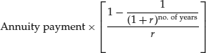
where r is the annual discount rate.
Applying this formula to a semiannual-pay bond, the annuity payment is one half the annual coupon payment and the number of periods is double the number of years to maturity. Accordingly, the present value of the coupon payments can be expressed as:
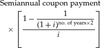
where i is the semiannual discount rate (r/2). Notice that in the formula, for the number of periods we use the number of years multiplied by 2 since a period in our illustration is six months.
The present value of the maturity value is just the present value of a lump sum and is equal to:

We will illustrate the calculation by valuing our 4-year, 6% coupon bond assuming that the relevant discount rate is 7%. The data are summarized below:

The present value of the coupon payments is:

This number tells us that the coupon payments contribute $20.6219 to the bond's value.
The present value of the maturity value is:

This number ($75.9412) tells us how much the maturity value contributes to the bond's value. The bond's value is then $96.5631 ($20.6219 + $75.9412). The price is less than par value and the bond is said to be trading at a discount. This will occur when the fixed coupon rate a bond offers (6%) is less than the required yield demanded by the market (the 7% discount rate). A discount bond has an inferior coupon rate relative to new comparable bonds being issued at par so its price must drop so as to offer the required yield of 7%. If the discount bond is held to maturity, the investor will experience a capital gain that just offsets the lower current coupon rate so that it appears equally attractive to new comparable bonds issued at par.
Suppose instead of a 7% discount rate, a 5% discount rate is used. This discount rate is less than the coupon rate on the bond (6%). It can be shown that the present value of the coupon payments is $21.5104 and the present value of the maturity value is $82.0747. Thus, the bond's value in this case is $103.5851. That is, the price is greater than par value and the bond is said to be trading at a premium. This will occur when the fixed coupon rate a bond offers (6%) is greater than the required yield demanded by the market (the 5% discount rate). Accordingly, a premium bond carries a higher coupon rate than new bonds (otherwise the same) being issued today at par so the price will be bid up and the required yield will fall until it equals 5%. If the premium bond is held to maturity, the investor will experience a capital loss that just offsets the benefits of the higher coupon rate so that it will appear equally attractive to new comparable bonds issued at par.
Finally, let's suppose that the discount rate is equal to the coupon rate. That is, suppose that the discount rate is 6%. It can be shown that the present value of the coupon payments is $21.0591 and the present value of the maturity value is $78.9409. Thus, the bond's value in this case is $100 or par value. Thus, when a bond's coupon rate is equal to the discount rate, the bond will trade at par value. Note that the preceding statement is strictly true only when a bond is valued on its coupon payment dates.
Valuing a Zero-Coupon Bond
For a zero-coupon bond, there is only one cash flow—the repayment of principal at maturity. The value of a zero-coupon bond that matures N years from now is:
![]()
where i is the semiannual discount rate.
The expression presented above states that the price of a zero-coupon bond is simply the present value of the maturity value. In the present value computation, why is the number of periods used for discounting rather than the number of years to the bond's maturity when there are no semiannual coupon payments? We do this in order to make the valuation of a zero-coupon bond consistent with the valuation of a coupon bond. In other words, both coupon and zero-coupon bonds are valued using semiannual discounting rates.
To illustrate, the value of a 10-year zero-coupon bond with a maturity value of $100 discounted at a 6.4% interest rate is $53.2606, as presented below:

Valuing a Bond between Coupon Payments
In our discussion of bond valuation to this point, we have assumed that the bonds are valued on their coupon payment dates (that is, the next coupon payment is one full period away). For bonds with semiannual coupon payments, this occurs only twice a year. Our task now is to describe how bonds are valued on the other 363 days (or 364 days) of the year.
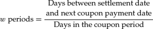
In order to value a bond with a settlement date between coupon payments, we must answer three questions. First, how many days are there until the next coupon payment date? The answer depends on the day count convention for the bond being valued. Second, how should we compute the present value of the cash flows received over the fractional period? Third, how much must the buyer compensate the seller for the coupon earned over the fractional period? This amount is accrued interest. We will answer these three questions in order to determine the full price and the clean price of a coupon bond. For a more detailed discussion of these issues for not only U.S. bonds but bonds traded in other countries, see Krgin (2002).
Computing the Full Price
When valuing a bond purchased with a settlement date between coupon payment dates, the first step is to determine the fractional periods between the settlement date and the next coupon date. Using the appropriate day count convention, this is determined as follows:
Then the present value of each expected future cash flow to be received t periods from now using a discount rate i assuming the next coupon payment is w periods from now (settlement date) is:
![]()
Note for the first coupon payment subsequent to the settlement date, t = 1 so the exponent is just w. This procedure for calculating the present value when a bond is purchased between coupon payments is called the “Street method.” In the Street method, as can be seen in the previous expression, coupon interest is compounded over the fractional period w.2
To illustrate the calculation, suppose that a U.S. Treasury note maturing on December 31, 2007, was purchased with a settlement date of November 22, 2006. This note's coupon rate was 4.375 and it had coupon payment dates of June 30 and December 31. As a result, the next coupon payment was December 31, 2006, while the previous coupon payment was paid on June 30, 2006. There were three cash flows remaining and they were to be delivered on December 31, 2006, June 30, 2007, and December 31, 2007. The final cash flow represented the last coupon payment and the maturity value of $100. Also assume the following:
Then w is 0.2120 periods (39/184). The present value of each cash flow assuming that each is discounted at a 4.9% annual discount rate is
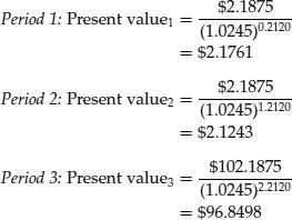
The sum of the present values of the cash flows is $101.1502. This price is referred to as the full price (or the dirty price).
It is the full price the bond's buyer pays the seller at delivery. However, the very next cash flow received and included in the present value calculation was not earned by the bond's buyer. A portion of the next coupon payment is the accrued interest. Accrued interest is the portion of a bond's next coupon payment that the bond's seller is entitled to depending on the amount of time the bond was held by the seller. Recall that the buyer recovers the accrued interest when the next coupon payment is delivered.
Computing the Accrued Interest and the Clean Price
The last step in this process is to find the bond's value without accrued interest (called the clean price or simply price). To do this, the accrued interest must be computed. The first step is to determine the number of days in the accrued interest period (that is, the number of days between the last coupon payment date and the settlement date) using the appropriate day count convention. For ease of exposition, we will assume in the example that follows that the actual/actual calendar is used. We will also assume there are only two bondholders in a given coupon period—the buyer and the seller.
As an illustration, we return to the previous example with the 4.375% coupon Treasury note. Since there were 184 days in the coupon period and 39 days from the settlement date to the next coupon period, there were 145 days (184−39) in the accrued interest period. Therefore, the percentage of the next coupon payment that is accrued interest is:
![]()
Of course, this is the same percentage found by simply subtracting w from 1. In our example, w was 0.2120. Then, 1 − 0.2120 = 0.7880.
Given the value of w, the amount of accrued interest (AI) is equal to:
![]()
Accordingly, using a 4.375 Treasury note with a settlement date of November 22, 2006, the portion of the next coupon payment that was accrued interest was:
![]()
Once we know the full price and the accrued interest, we can determine the clean price. The clean price is the price quoted in the market and represents the bond's value to the new bondholder. The clean price is computed as follows:
![]()
In our illustration, the clean price is:
![]()
Note that in computing the full price, the present value of the next coupon payment is computed. However, the buyer pays the seller the accrued interest now despite the fact that it will not be recovered until the next coupon payment date. To make this concrete, suppose one sells a bond such that the settlement date is halfway between the coupon payment dates. In this case w = 0.50. Accordingly, the seller will be entitled to one-half of the next coupon payment which would not otherwise be received for another three months. Thus, when calculating the clean price, we subtract “too much” accrued interest—one-half the coupon payment rather than the present value of one-half the coupon payment. Of course, this is the market convention for calculating accrued interest but it does introduce a curious twist in bond valuation.
The Price/Discount Rate Relationship
An important general property of present value is that the higher (lower) the discount rate, the lower (higher) the present value. Since the value of a security is the present value of the expected future cash flows, this property carries over to the value of a security: The higher (lower) the discount rate, the lower (higher) a security's value. We can summarize the relationship between the coupon rate, the required market yield, and the bond's price relative to its par value as follows:
![]()

This agrees with what we found for the 4-year, 6% coupon bond:

Figure 1 depicts this inverse relationship between an option-free bond's price and its discount rate (that is, required yield). There are two things to infer from the price/discount rate relationship depicted in the figure. First, the relationship is downward sloping. This is simply the inverse relationship between present values and discount rates at work. Second, the relationship is represented as a curve rather than a straight line. In fact, the shape of the curve in Figure 1 is referred to as convex. By convex, it simply means the curve is “bowed in” relative to the origin. This second observation raises two questions about the convex or curved shape of the price/discount rate relationship. First, why is it curved? Second, what is the import of the curvature?
Figure 1 Price/Discount Rate Relationship for an Option-Free Bond
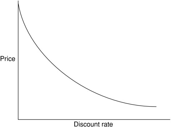
The answer to the first question is mathematical. The answer lies in the denominator of the bond pricing formula. Since we are raising one plus the discount rate to powers greater than one, it should not be surprising that the relationship between the level of the price and the level of the discount rate is not linear.
As for the importance of the curvature to bond investors, let's consider what happens to bond prices in both falling and rising interest rate environments. First, what happens to bond prices as interest rates fall? The answer is obvious—bond prices rise. How about the rate at which they rise? If the price/discount rate relationship was linear, as interest rates fell, bond prices would rise at a constant rate. However, the relationship is not linear, it is curved and curved inward. Accordingly, when interest rates fall, bond prices increase at an increasing rate. Now, let's consider what happens when interest rates rise. Of course, bond prices fall. How about the rate at which bond prices fall? Once again, if the price/discount rate relationship were linear, as interest rates rose, bond prices would fall at a constant rate. Since it curved inward, when interest rates rise, bond prices decrease at a decreasing rate.
Time Path of Bond
As a bond moves towards its maturity date, its value changes. More specifically, assuming that the discount rate does not change, a bond's value:
With respect to the last property, we are assuming the bond is valued on its coupon anniversary dates.
At the maturity date, the bond's value is equal to its par or maturity value. So, as a bond's maturity approaches, the price of a discount bond will rise to its par value and a premium bond will fall to its par value—a characteristic sometimes referred to as pull to par value.
ARBITRAGE-FREE BOND VALUATION
The traditional approach to valuation is to discount every cash flow of a fixed income security using the same interest or discount rate. The fundamental flaw of this approach is that it views each security as the same package of cash flows. For example, consider a 5-year U.S. Treasury note with a 6% coupon rate. The cash flows per $100 of par value would be 9 payments of $3 every six months and $103 ten 6-month periods from now. The traditional practice would discount every cash flow using the same discount rate regardless of when the cash flows are delivered in time and the shape of the yield curve. Finance theory tells us that any security should be thought of as a package or portfolio of zero-coupon bonds.
The proper way to view the 5-year 6% coupon Treasury note is as a package of zero-coupon instruments whose maturity value is the amount of the cash flow and whose maturity date coincides with the date the cash flow is to be received. Thus, the 5-year 6% coupon Treasury issue should be viewed as a package of 10 zero-coupon instruments that mature every six months for the next five years. This approach to valuation does not allow a market participant to realize an arbitrage profit by breaking apart or “stripping” a bond and selling the individual cash flows (that is, stripped securities) at a higher aggregate value than it would cost to purchase the security in the market. Simply put, arbitrage profits are possible when the sum of the parts is worth more than the whole or vice versa. Because this approach to valuation precludes arbitrage profits, we refer to it as the arbitrage-free valuation approach.
By viewing any security as a package of zero-coupon bonds, a consistent valuation framework can be developed. Viewing a security as a package of zero-coupon bonds means that two bonds with the same maturity and different coupon rates are viewed as different packages of zero-coupon bonds and valued accordingly. Moreover, two cash flows that have identical risk delivered at the same time will be valued using the same discount rate even though they are attached to two different bonds.
To implement the arbitrage-free approach it is necessary to determine the theoretical rate that the U.S. Treasury would have to pay on a zero-coupon Treasury security for each maturity. We say “theoretical” because other than U.S. Treasury bills, the Treasury does not issue zero-coupon bonds. Zero-coupon Treasuries are, however, created by dealer firms. The name given to the zero-coupon Treasury rate is the (Treasury) spot rate. Our next task is to explain how the Treasury spot rate can be calculated.
Theoretical Spot Rates
The theoretical spot rates for Treasury securities represent the appropriate set of interest or discount rates that should be used to value default-free cash flows. A default-free theoretical spot rate can be constructed from the observed Treasury yield curve or par curve. We will begin our quest of how to estimate spot rates with the par curve.
Par Rates
The raw material for all yield curve analysis is the set of yields on the most recently issued (that is, on-the-run) Treasury securities. The U.S. Treasury routinely issues 10 securities—the 1-month, 3-month, 6-month, and 1-year bills and the 2-, 3-, 5-, 7-, and 10-year notes, and a 30-year bond. These on-the-run Treasury issues are default risk-free and trade in one of the most liquid and efficient secondary markets in the world. Because of these characteristics, historically Treasury yields serve as a reference benchmark for risk-free rates which are used for pricing other securities. However, other benchmarks such as the swap curve are now used but the principles of valuation remain unchanged.
In practice, however, the observed yields for the on-the-run Treasury coupon issues are not usually used directly. Instead, the coupon rate is adjusted so that the price of the issue would be the par value. Accordingly, the par yield curve is the adjusted on-the-run Treasury yield curve where coupon issues are at par value and the coupon rate is therefore equal to the yield to maturity. The exception is for the 6-month Treasury bills; the bond-equivalent yield for this issue is already the spot rate.
Deriving a par curve from a set of points starting with the yield on the 6-month bill and ending the yield on the 30-year bond is not a trivial matter. The end result is a curve that tells us “if the Treasury were to issue a security today with a maturity equal to say 12 years, what coupon rate would the security have to pay in order to sell at par?” Some analysts contend that estimating the par curve with only the yields of the on-the-run Treasuries uses too little information that is available from the market. In particular, one must estimate the back-end of the yield curve with only one security, that is, the 30-year bond. Some analysts prefer to use the on-the-run Treasuries and selected off-the-run Treasuries.
In summary, a par rate is the average discount rate of many cash flows (those of a par bond) over many periods. This begs the question, “the average of what?” As we will see, par rates are complicated averages of the implied spot rates. Thus, in order to uncover the spot rates, we must find a method to “break apart” the par rates. There are several approaches that are used in practice.3 The approach that we describe below for creating a theoretical spot rate curve is called bootstrapping.
Bootstrapping the Spot Rate Curve
Bootstrapping begins with the par curve. To illustrate bootstrapping, we will use the Treasury par curve shown in Table 1. The par yield curve shown extends only out to 10 years. Our objective is to show how the values in the last column of the table (labeled “Spot Rate”) are obtained. Throughout the analysis and illustrations to come, it is important to remember the basic principle is that the value of the Treasury coupon security should be equal to the value of the package of zero-coupon Treasury securities that duplicates the coupon bond's cash flows.
Table 1 Hypothetical Treasury Par Yield Curve

The key to this process is the existence of the Treasury strips market. A government securities dealer has the ability to take apart the cash flows of a Treasury coupon security (that is, strip the security) and create zero-coupon securities. These zero-coupon securities, which are called Treasury strips, can be sold to investors. At what interest rate or yield can these Treasury strips be sold to investors? The answer is they can be sold at the Treasury spot rates. If the market price of a Treasury security is less than its value after discounting with spot rates (that is, the sum of the parts is worth more than the whole), then a dealer can buy the Treasury security, strip it, and sell off the Treasury strips so as to generate greater proceeds than the cost of purchasing the Treasury security. The resulting profit is an arbitrage profit.
Before we proceed to our illustration of bootstrapping, a very sensible question must be addressed. Specifically, if Treasury strips are in effect zero-coupon Treasury securities, why not use strip rates (that is, the rates on Treasury strips) as our spot rates? In other words, why must we estimate theoretical spot rates via bootstrapping using yields from Treasury bills, notes, and bonds when we already have strip rates conveniently available? There are three major reasons. First, although Treasury strips are actively traded, they are not as liquid as on-the-run Treasury bills, notes, and bonds. As a result, Treasury strips have some liquidity risk for which investors will demand some compensation in the form of higher yields. Second, the tax treatment of strips is different from that of Treasury coupon securities. Specifically, the accrued interest on strips is taxed even though no cash is received by the investor. Thus, they are negative cash flow securities to taxable entities, and, as a result, their yield reflects this tax disadvantage. Finally, there are maturity sectors where non-U.S. investors find it advantageous to trade off yield for tax advantages associated with a strip. Specifically, certain non-U.S. tax authorities allow their citizens to treat the difference between the maturity value and the purchase price as a capital gain and tax this gain at a favorable tax rate. Some will grant this favorable treatment only when the strip is created from the principal rather than the coupon. For this reason, those who use Treasury strips to represent theoretical spot rates restrict the issues included to coupon strips.
Now let's see how to generate the spot rates. Consider the 6-month Treasury security in Table 1. This security is a Treasury bill and is issued as a zero-coupon instrument. Therefore, the annualized bond-equivalent yield (not the bank discount yield) of 3.00% for the 6-month Treasury security is equal to the 6-month spot rate. Using the yield on the 1-year bill, we use 3.3% as the 1-year spot rate. Given these two spot rates, we can compute the spot rate for a theoretical 1.5-year zero-coupon Treasury. The value of a theoretical 1.5-year Treasury should equal the present value of the three cash flows from the 1.5-year coupon Treasury, where the yield used for discounting is the spot rate corresponding to the time of receipt of the cash flow. Since all the coupon bonds are selling at par, as explained in the previous section, the yield to maturity for each bond is the coupon rate. Using $100 as par, the cash flows for the 1.5-year coupon Treasury are:

The present value of the cash flows is then:
![]()
where
z1 = one-half the annualized 6-month theoretical spot rate
z2 = one-half the 1-year theoretical spot rate
z3 = one-half the 1.5-year theoretical spot rate
Since the 6-month spot rate is 3% and the 1-year spot rate is 3.30%, we know that:
![]()
We can compute the present value of the 1.5-year coupon Treasury security as:

Since the price of the 1.5-year coupon Treasury security is equal to its par value (see Table 1), the following relationship must hold
![]()
If we had not been working with a par yield curve, the equation would have been set to the market price for the 1.5-year issue rather than par value.
Note we are treating the 1.5 year par bond as if it were a portfolio of three zero-coupon bonds. Moreover, each cash flow has its own discount rate that depends on when the cash flow is delivered in the future and the shape of the yield curve. This is in sharp contrast to the traditional valuation approach that forces each cash flow to have the same discount rate.
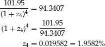
We can solve for the theoretical 1.5-year spot rate as follows:

Doubling this yield we obtain the bond-equivalent yield of 3.5053%, which is the theoretical 1.5-year spot rate. This is the rate that the market would apply to a 1.5-year zero-coupon Treasury security if, in fact, such a security existed. In other words, all Treasury cash flows to be received 1.5 years from now should be valued (that is, discounted) at 3.5053%.
Given the theoretical 1.5-year spot rate, we can obtain the theoretical 2-year spot rate. The cash flows for the 2-year coupon Treasury in Table 1 are:

The present value of the cash flows is then:
![]()
where z4 = one-half of the 2-year theoretical spot rate.
Since the 6-month spot rate, 1-year spot rate, and 1.5-year spot rate are 3.00%, 3.30%, and 3.5053%, respectively, then:
![]()
Therefore, the present value of the 2-year coupon Treasury security is:

Since the price of the 2-year coupon Treasury security is equal to par, the following relationship must hold:

We can solve for the theoretical 2-year spot rate as follows:
Doubling this yield, we obtain the theoretical 2-year spot rate bond-equivalent yield of 3.9164%.
One can follow this approach sequentially to derive the theoretical 2.5-year spot rate from the calculated values of z1, z2, z3, and z4 (the 6-month, 1-year, 1.5-year, and 2-year rates), and the price and coupon of the 2.5-year bond in Table 1. Further, one could derive theoretical spot rates for the remaining 15 half-yearly rates. The spot rates thus obtained are shown in the last column of Table 1. They represent the term structure of default-free spot rate for maturities up to 10 years at the particular time to which the bond price quotations refer.
Let us summarize to this point. We started with the par curve which is constructed using the adjusted yields from the on-the-run Treasuries. A par rate is the average discount rate of many cash flows over many periods. Specifically, par rates are complicated averages of spot rates. The spot rates are uncovered from par rates via bootstrapping. A spot rate is the average discount rate of a single cash flow over many periods. It appears that spot rates are also averages. Spot rates are averages of one or more forward rates.
Valuation Using Treasury Spot Rates
To illustrate how Treasury spot rates are used to compute the arbitrage-free value of a Treasury security, we will use the hypothetical Treasury spot rates shown in the fourth column of Table 2 to value an 8%, 10-year Treasury security. The present value of each period's cash flow is shown in the fifth column. The sum of the present values is the arbitrage-free value for the Treasury security. For the 8%, 10-year Treasury it is $107.0018.
Table 2 Determination of the Arbitrage-Free Value of an 8% 10-Year Treasury and Arbitrage Opportunity

Reason for Using Treasury Spot Rates
Thus far, we have simply asserted that the value of a Treasury security should be based on discounting each cash flow using the corresponding Treasury spot rate. But what if market participants value a security using just the yield for the on-the-run Treasury with a maturity equal to the maturity of the Treasury security being valued? Let's see why the value of a Treasury security should trade close to its arbitrage-free value.
Stripping and Arbitrage-Free Valuation
The key to the arbitrage-free valuation approach is the existence of the Treasury strips market. A dealer has the ability to take apart the cash flows of a Treasury coupon security (that is, strip the security) and create zero-coupon securities. These zero-coupon securities, called Treasury strips, can be sold to investors. At what interest rate or yield can these Treasury strips be sold to investors? They can be sold at the Treasury spot rates. If the market price of a Treasury security is less than its value using the arbitrage-free valuation approach, then a dealer can buy the Treasury security, strip it, and sell off the individual Treasury strips so as to generate greater proceeds than the cost of purchasing the Treasury security. The resulting profit is an arbitrage profit. Since as we will see, the value determined by using the Treasury spot rates does not allow for the generation of an arbitrage profit, this is referred to as an “arbitrage-free” approach.
To illustrate this, suppose that the yield for the on-the-run 10-year Treasury issue is 7.08%. Suppose that the 8% coupon 10-year Treasury issue is valued using the traditional approach based on 7.08%. The value based on discounting all the cash flows at 7.08% is $106.5141 as shown in the next-to-the-last column in Table 2.
Consider what would happen if the market priced the security at $106.5141 and that the spot rates are those shown in the fourth column of Table 2. The value based on the Treasury spot rates is $107.0018 as shown in the fifth column of Table 2. What can the dealer do? The dealer can buy the 8% 10-year issue for $106.5141, strip it, and sell the Treasury strips at the spot rates shown in Table 2. By doing so, the proceeds that will be received by the dealer are $107.0018. This results in an arbitrage profit (ignoring transaction costs) of $0.4877 (= $107.0018 − $106.5141). Dealers recognizing this arbitrage opportunity will bid up the price of the 8% 10-year Treasury issue in order to acquire it and strip it. The arbitrage profit will be eliminated when the security is priced at $107.0018, the value that we said is the arbitrage-free value.
To understand in more detail where this arbitrage profit is coming from, look at the last three columns in Table 2. The sixth column shows how much each cash flow can be sold for by the dealer if it is stripped. The values in this column are just those in the fifth column. The next-to-last column shows how much the dealer is effectively purchasing the cash flow for if each cash flow is discounted at 7.08%. The sum of the arbitrage profit from each stripped cash flow is the total arbitrage profit and is contained in the last column.
We have just demonstrated how coupon stripping of a Treasury issue will force the market value to be close to the value as determined by the arbitrage-free valuation approach when the market price is less than the arbitrage-free value (that is, the whole is worth less than the sum of the parts). What happens when a Treasury issue's market price is greater than the arbitrage-free value? Obviously, a dealer will not want to strip the Treasury issue since the proceeds generated from stripping will be less than the cost of purchasing the issue.
When such situations occur, the dealer can purchase a package of Treasury strips so as to create a synthetic Treasury coupon security that is worth more than the same maturity and same coupon Treasury issue. This process is called reconstitution.
The process of stripping and reconstituting ensures that the price of a Treasury issue will not depart materially (depending on transaction costs) from its arbitrage-free value.
Credit Spreads and the Valuation of Non-Treasury Securities
The Treasury spot rates can be used to value any default-free security. For a non-Treasury security, the theoretical value is not as easy to determine. The value of a non-Treasury security is found by discounting the cash flows by the Treasury spot rates plus a yield spread which reflects the additional risks (e.g., default risk, liquidity risks, the risk associated with any embedded options, and so on).
The spot rate used to discount the cash flow of a non-Treasury security can be the Treasury spot rate plus a constant credit spread. For example, suppose the 6-month Treasury spot rate is 6.05% and the 10-year Treasury spot rate is 7.20%. Also suppose that a suitable credit spread is 100 basis points. Then a 7.05% spot rate is used to discount a 6-month cash flow of a non-Treasury bond and an 8.20% discount rate is used to discount a 10-year cash flow. (Remember that when each semiannual cash flow is discounted, the discount rate used is one-half the spot rate: 3.525% for the 6-month spot rate and 4.10% for the 10-year spot rate.)
The drawback of this approach is that there is no reason to expect the credit spread to be the same regardless of when the cash flow is expected to be received. Consequently, the credit spread may vary with a bond's term to maturity. In other words, there is a term structure of credit spreads. Generally, credit spreads increase with maturity. This is a typical shape for the term structure of credit spreads. Moreover, the shape of the term structure is not the same for all credit ratings. Typically, the lower the credit rating, the steeper the term structure of credit spreads.
Dealer firms typically estimate the term structure of credit spreads for each credit rating and market sector. Typically, the credit spread increases with maturity. In addition, the shape of the term structure is not the same for all credit ratings. Typically, the lower the credit rating, the steeper the term structure of credit spreads.
Table 3 Calculation of Arbitrage-Free Value of a Hypothetical 8% 10-Year Non-Treasury Security Using Benchmark Spot Rate Curve
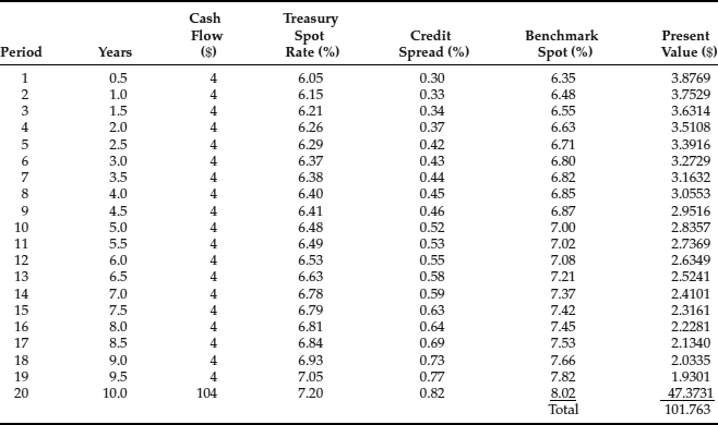
When the relevant credit spreads for a given credit rating and market sector are added to the Treasury spot rates, the resulting term structure is used to value the bonds of issuers with that credit rating in that market sector. This term structure is referred to as the benchmark spot rate curve or benchmark zero-coupon rate curve.
For example, Table 3 reproduces the Treasury spot rate curve in Table 2. Also shown is a hypothetical term structure of credit spreads for a non-Treasury security. The resulting benchmark spot rate curve is in the next-to-the-last column. Like before, it is this spot rate curve that is used to value the securities of issuers that have the same credit rating and are in the same market sector. This is done in Table 3 for a hypothetical 8% 10-year issue. The arbitrage-free value is $101.763. Notice that the theoretical value is less than that for an otherwise comparable Treasury security. The arbitrage-free value for an 8% 10-year Treasury is $107.0018 (see Table 3).
KEY POINTS
- A bond can be thought of as a portfolio or package of cash flows. Accordingly, the value of a bond is simply the present value of its remaining expected future cash flows.
- There is an inverse relationship between bond prices/required yields.
- The traditional approach to valuation is to discount each cash flow with the same discount rate. The weakness of the traditional approach is its reliance on using the same discount rate for all of the bond's cash flows.
- The arbitrage-free approach allows each cash flow to be valued as a zero-coupon bond with a discount rate that depends on the shape of the yield curve and when the cash flow is delivered in time.
- The bootstrapping technique is used to derive the discount rates for discounting a bond's cash flows. These discount rates are called spot rates.
- Default-free bonds should trade at prices close to their arbitrage-free values. The process of stripping and reconstituting of Treasury securities ensures that this will occur.
NOTES
1. For a description of these securities, see Fabozzi (2012).
2. There is another method called the “Treasury method,” which treats the coupon interest over the fractional period as simple interest.
3. There is an extensive literature on estimating spot rates or what is known as term structure modeling. See Fabozzi (2002).
REFERENCES
Fabozzi, F.J. (2012). Bond Markets, Analysis, and Strategies: 8ed. Hoboken, NJ: John Wiley & Sons.
Fabozzi, F.J. (ed.) (2002). Interest Rate, Term Structure, and Valuation Modeling. Hoboken, NJ: John Wiley & Sons.
Krgin, D. (2002). Handbook of Global Fixed Income Calculations. Hoboken, NJ: John Wiley & Sons.