
Modeling Market Impact Costs
Trading is an integral component of the equity investment process. A poorly executed trade can eat directly into portfolio returns. This is because equity markets are not frictionless, and transactions have a cost associated with them. Costs are incurred when buying or selling stocks in the form of, for example, brokerage commissions, bid-ask spreads, taxes, and market impact costs.
In recent years, portfolio managers have started to more carefully consider transaction costs. The literature on market microstructure, analysis and measurement of transaction costs, and market impact costs on institutional trades is rapidly expanding.1 One way of describing transaction costs is to categorize them in terms of explicit costs such as brokerage and taxes, and implicit costs, which include market impact costs, price movement risk, and opportunity cost. Market impact cost is, broadly speaking, the price an investor has to pay for obtaining liquidity in the market, whereas price movement risk is the risk that the price of an asset increases or decreases from the time the investor decides to transact in the asset until the transaction actually takes place. Opportunity cost is the cost suffered when a trade is not executed. Another way of seeing transaction costs is in terms of fixed costs versus variable costs. Whereas commissions and trading fees are fixed, bid-ask spreads, taxes, and all implicit transaction costs are variable.
Portfolio managers and traders need to be able to effectively model the impact of trading costs on their portfolios and trades. In this entry, we introduce several approaches for the modeling of transaction costs, in particular market impact costs.
MARKET IMPACT COSTS
The market impact cost of a transaction is the deviation of the transaction price from the market (mid) price2 that would have prevailed had the trade not occurred. The price movement is the cost, the market impact cost, for liquidity. Market impact of a trade can be negative if, for example, a trader buys at a price below the no-trade price (i.e., the price that would have prevailed had the trade not taken place). In general, liquidity providers experience negative costs while liquidity demanders will face positive costs.
We distinguish between two different kinds of market impact costs, temporary and permanent. Total market impact cost is computed as the sum of the two. The temporary market impact cost is of transitory nature and can be seen as the additional liquidity concession necessary for the liquidity provider (e.g., the market maker) to take the order, inventory effects (price effects due to broker/dealer inventory imbalances), or imperfect substitution (for example, price incentives to induce market participants to absorb the additional shares).
The permanent market impact cost, however, reflects the persistent price change that results as the market adjusts to the information content of the trade. Intuitively, a sell transaction reveals to the market that the security may be overvalued, whereas a buy transaction signals that the security may be undervalued. Security prices change when market participants adjust their views and perceptions as they observe news and the information contained in new trades during the trading day.
Traders can decrease the temporary market impact by extending the trading horizon of an order. For example, a trader executing a less urgent order can buy or sell his or her position in smaller portions over a period and make sure that each portion only constitutes a small percentage of the average volume. However, this comes at the price of increased opportunity costs, delay costs, and price movement risk.
Market impact costs are often asymmetric; that is, they are different for buy and sell orders. Several empirical studies suggest that market impact costs are generally higher for buy orders. Nevertheless, while buying costs might be higher than selling costs, this empirical fact is most likely due to observations during rising/falling markets, rather than any true market microstructure effects. For example, a study by Hu shows that the difference in market impact costs between buys and sells is an artifact of the trade benchmark.3 (We discuss trade benchmarks later in this entry.) When a pre-trade measure is used, buys (sells) have higher implicit trading costs during rising (falling) markets. Conversely, if a post-trade measure is used, sells (buys) have higher implicit trading costs during rising (falling) markets. In fact, both pre-trade and post-trade measures are highly influenced by market movement, whereas during- or average-trade measures are neutral to market movement.
Despite the enormous global size of equity markets, the impact of trading is important even for relatively small funds. In fact, a sizable fraction of the stocks that compose an index might have to be excluded or their trading severely limited. For example, RAS Asset Management, which is the asset manager arm of the large Italian insurance company RAS, has determined that single trades exceeding 10% of the daily trading volume of a stock cause an excessive market impact and have to be excluded, while trades between 5% and 10% need execution strategies distributed over several days.4 According to RAS Asset Management estimates, in practice funds managed actively with quantitative techniques and with market capitalization in excess of €100 million can operate only on the fraction of the market above the €5 million, splitting trades over several days for stocks with average daily trading volume in the range from €5 million to €10 million. They can freely operate only on two-thirds of the stocks in the MSCI Europe.
LIQUIDITY AND TRANSACTION COSTS
Liquidity is created by agents transacting in the financial markets when they buy and sell securities. Market makers and brokers–dealers do not create liquidity; they are intermediaries who facilitate trade execution and maintain an orderly market.
Liquidity and transaction costs are interrelated. A highly liquid market is one where large transactions can be immediately executed without incurring high transaction costs. In an indefinitely liquid market, traders would be able to perform very large transactions directly at the quoted bid-ask prices. In reality, particularly for larger orders, the market requires traders to pay more than the ask when buying and to receive less than the bid when selling. As we discussed previously, this percentage degradation of the bid-ask prices experienced when executing trades is the market impact cost.
The market impact cost varies with transaction size: The larger the trade size, the larger the impact cost. Impact costs are not constant in time, but vary throughout the day as traders change the limit orders that they have in the limit order book. A limit order is a conditional order; it is executed only if the limit price or a better price can be obtained. For example, a buy limit order of a security XYZ at $60 indicates that the assets may be purchased only at $60 or lower. Therefore, a limit order is very different from a market order, which is an unconditional order to execute at the current best price available in the market (guarantees execution, not price). With a limit order, a trader can improve the execution price relative to the market order price, but the execution is neither certain nor immediate (guarantees price, not execution).
Notably, there are many different limit order types available such as pegging orders, discretionary limit orders, immediate or cancel order (IOC) orders, and fleeting orders. For example, fleeting orders are those limit orders that are canceled within two seconds of submission. Hasbrouck and Saar find that fleeting limit orders are much closer substitutes for market orders than for traditional limit orders.5 This suggests that the role of limit orders has changed from the traditional view of being liquidity suppliers to being substitutes for market orders.
At any given instant, the list of orders sitting in the limit order book embodies the liquidity that exists at a particular point in time. By observing the entire limit order book, impact costs can be calculated for different transaction sizes. The limit order book reveals the prevailing supply and demand in the market.6 Therefore, in a pure limit order market, we can obtain a measure of liquidity by aggregating limit buy orders (representing the demand) and limit sell orders (representing the supply).7
We start by sorting the bid and ask prices, ![]() and
and ![]() (from the most to the least competitive) and the corresponding order quantities
(from the most to the least competitive) and the corresponding order quantities ![]() and
and ![]() . We then combine the sorted bid and ask prices into a supply and demand schedule according to Figure 1. For example, the block (
. We then combine the sorted bid and ask prices into a supply and demand schedule according to Figure 1. For example, the block (![]() ) represents the second best sell limit order with price
) represents the second best sell limit order with price ![]() and quantity
and quantity ![]() .
.
Figure 1 The Supply and Demand Schedule of a Security
Source: Figure 1A in Domowitz and Wang (2002, p. 38).
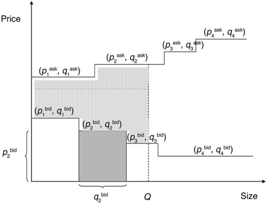
We note that unless there is a gap between the bid (demand) and the ask (supply) sides, there will be a match between a seller and buyer, and a trade would occur. The larger the gap, the lower the liquidity and the market participants’ desire to trade. For a trade of size Q, we can define its liquidity as the reciprocal of the area between the supply and demand curves up to Q (i.e., the “dotted” area in Figure 1).
However, few order books are publicly available and not all markets are pure limit order markets. In 2004, the New York Stock Exchange (NYSE) started selling information on its limit order book through its new system called the NYSE OpenBook®. The system provides an aggregated real-time view of the exchange's limit-order book for all NYSE-traded securities.8
In the absence of a fully transparent limit order book, expected market impact cost is the most practical and realistic measure of market liquidity. It is closer to the true cost of transacting faced by market participants as compared to other measures such as those based upon the bid-ask spread.
MARKET IMPACT MEASUREMENTS AND EMPIRICAL FINDINGS
The problem with measuring implicit transaction costs is that the true measure, which is the difference between the price of the stock in the absence of a money manager's trade and the execution price, is not observable. Furthermore, the execution price is dependent on supply and demand conditions at the margin. Thus, the execution price may be influenced by competitive traders who demand immediate execution or by other investors with similar motives for trading. This means that the execution price realized by an investor is the consequence of the structure of the market mechanism, the demand for liquidity by the marginal investor, and the competitive forces of investors with similar motivations for trading.
There are many ways to measure transaction costs. However, in general this cost is the difference between the execution price and some appropriate benchmark, a so-called fair market benchmark. The fair market benchmark of a security is the price that would have prevailed had the trade not taken place, the no-trade price. Since the no-trade price is not observable, it has to be estimated. Practitioners have identified three different basic approaches to measure the market impact:9
The volume-weighted average price is calculated as follows. Suppose that it was a trader's objective to purchase 10,000 shares of stock XYZ. After completion of the trade, the trade sheet showed that 4,000 shares were purchased at $80, another 4,000 at $81, and finally 2,000 at $82. In this case, the resulting VWAP is (4,000 × 80 + 4,000 × 81 + 2,000 × 82)/10,000 = $80.80.
We denote by χ the indicator function that takes on the value 1 or −1 if an order is a buy or sell order, respectively. Formally, we now express the three types of measures of market impact (MI) as follows
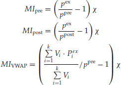
where pex, ppre, and ppost denote the execution price, pre-trade price, and post-trade price of the stock, and k denotes the number of transactions in a particular security on the trade date. Using this definition, for a stock with market impact MI the resulting market impact cost for a trade of size V, MIC, is given by
![]()
It is also common to adjust market impact for general market movements. For example, the pre-trade market impact with market adjustment would take the form
![]()
where ![]() represent the value of the index at the time of the execution, and
represent the value of the index at the time of the execution, and ![]() the price of the index at the time before the trade. Market-adjusted market impact for the post-trade and same-day trade benchmarks are calculated in an analogous fashion.
the price of the index at the time before the trade. Market-adjusted market impact for the post-trade and same-day trade benchmarks are calculated in an analogous fashion.
The above three approaches to measure market impact are based upon measuring the fair market benchmark of stock at a point in time. Clearly, different definitions of market impact lead to different results. Which one should be used is a matter of preference and is dependent on the application at hand. For example, Elkins and McSherry, a financial consulting firm that provides customized trading costs and execution analysis, calculates a same-day benchmark price for each stock by taking the mean of the day's open, close, high, and low prices. The market impact is then computed as the percentage difference between the transaction price and this benchmark. However, in most cases VWAP and the Elkins McSherry approach lead to similar measurements.11
As we analyze a portfolio's return over time an important question to ask is whether we can attribute good/bad performance to investment profits/losses or to trading profits/losses. In other words, in order to better understand a portfolio's performance it can be useful to decompose investment decisions from order execution. This is the basic idea behind the implementation shortfall approach suggested by Perold (1998).
In the implementation shortfall approach, we assume that there is a separation between investment and trading decisions. The portfolio manager makes decisions with respect to the investment strategy (i.e., what should be bought, sold, and held). Subsequently, these decisions are implemented by the traders.
By comparing the actual portfolio profit/loss (P/L) with the performance of a hypothetical paper portfolio in which all trades are made at hypothetical market prices, we can get an estimate of the implementation shortfall. For example, with a paper portfolio return of 6% and an actual portfolio return of 5%, the implementation shortfall is 1%.
There is considerable practical and academic interest in the measurement and analysis of international trading costs. Domowitz, Glen, and Madhavan (1999) examine international equity trading costs across a broad sample of 42 countries using quarterly data from 1995 to 1998. They find that the mean total one-way trading cost is 69.81 basis points. However, there is an enormous variation in trading costs across countries. For example, in their study the highest was Korea with 196.85 basis points whereas the lowest was France with 29.85 basis points. Explicit costs are roughly two-thirds of total costs. However, one exception to this is the United States where the implicit costs are about 60% of the total costs.
Transaction costs in emerging markets are significantly higher than those in more developed markets. Domowitz, Glen, and Madhavan argue that this fact limits the gains of international diversification in these countries, explaining in part the documented home bias of domestic investors.
In general, they find that transaction costs declined from the middle of 1997 to the end of 1998, with the exception of Eastern Europe. It is interesting to notice that this reduction in transaction costs happened despite the turmoil in the financial markets during this period. A few explanations that Domowitz et al. suggest are that (1) the increased institutional presence has resulted in a more competitive environment for brokers/dealers and other trading services; (2) technological innovation has led to a growth in the use of low-cost electronic crossing networks (ECNs) by institutional traders; and (3) soft dollar payments are now more common.
FORECASTING AND MODELING MARKET IMPACT
In this section, we describe a general methodology for constructing forecasting models for market impact. These types of models are very useful in predicting the resulting trading costs of specific trading strategies and in devising optimal trading approaches.
Explicit transaction costs are relatively straightforward to estimate and forecast. Therefore, our focus in this section is to develop a methodology for the implicit transaction costs, and more specifically, market impact costs. The methodology is a linear factor-based approach where market impact is the dependent variable. We distinguish between trade-based and asset-based independent variables or forecasting factors.
Trade-Based Factors
Some examples of trade-based factors include:
- Trade size
- Relative trade size
- Price of market liquidity
- Type of trade (information or informationless trade)
- Efficiency and trading style of the investor
- Specific characteristics of the market or the exchange
- Time of trade submission and trade timing
- Order type
Probably the most important market impact forecasting variables are based on absolute or relative trade size. Absolute trade size is often measured in terms of the number of shares traded, or the dollar value of the trade. Relative trade size, on the other hand, can be calculated as number of shares traded divided by average daily volume, or number of shares traded divided by the total number of shares outstanding. Note that the former can be seen as an explanatory variable for the temporary market impact and the latter for the permanent market impact. In particular, we expect the temporary market impact to increase as the trade size to the average daily volume increases because a larger trade demands more liquidity.
Each type of investment style requires a different need for immediacy.12 Technical trades often have to be traded at a faster pace in order to capitalize on some short-term signal and therefore exhibit higher market impact costs. In contrast, more traditional long-term value strategies can be traded more slowly. These types of strategies can in many cases even be liquidity providing, which might result in negative market impact costs.
Several studies show that there is a wide variation in equity transaction costs across different countries.13 Markets and exchanges in each country are different, and so are the resulting market microstructures. Forecasting variables can be used to capture specific market characteristics such as liquidity, efficiency, and institutional features.
The particular timing of a trade can affect the market impact costs. For example, it appears that market impact costs are generally higher at the beginning of the month as compared to the end of it.14 One of the reasons for this phenomenon is that many institutional investors tend to rebalance their portfolios at the beginning of the month. Because it is likely that many of these trades will be executed in the same stocks, this rebalancing pattern will induce an increase in market impact costs. The particular time of the day a trade takes place does also have an effect. Many informed institutional traders tend to trade at the market open as they want to capitalize on new information that appeared after the market close the day before.
As we discussed earlier in this entry, market impact costs are asymmetric. In other words, buy and sell orders have significantly different market impact costs. Separate models for buy and sell orders can therefore be estimated. However, it is now more common to construct a model that includes dummy variables for different types of orders such as buy/sell orders, market orders, limit orders, and the like.
Asset-Based Factors
Some examples of asset-based factors are:
- Price momentum
- Price volatility
- Market capitalization
- Growth versus value
- Specific industry or sector characteristics
For a stock that is exhibiting positive price momentum, a buy order is liquidity demanding and it is, therefore, likely that it will have higher market impact cost than a sell order.
Generally, trades in high volatility stocks result in higher permanent price effects. It has been suggested by Chan and Lakonishok (1997) and Smith et al. (2001) that this is because trades have a tendency to contain more information when volatility is high. Another possibility is that higher volatility increases the probability of hitting and being able to execute at the liquidity providers’ price. Consequently, liquidity suppliers display fewer shares at the best prices to mitigate adverse selection costs.
Large-cap stocks are more actively traded and therefore more liquid in comparison to small-cap stocks. As a result, market impact cost is normally lower for large caps.15 However, if we measure market impact costs with respect to relative trade size (normalized by average daily volume, for instance), they are generally higher. Similarly, growth and value stocks have different market impact cost. One reason for that is related to the trading style. Growth stocks commonly exhibit momentum and high volatility. This attracts technical traders that are interested in capitalizing on short-term price swings. Value stocks are traded at a slower pace and holding periods tend to be slightly longer.
Different market sectors show different trading behaviors. For instance, Bikker and Spierdijk (2007) show that equity trades in the energy sector exhibit higher market impact costs than other comparable equities in nonenergy sectors.
A Factor-Based Market Impact Model
One of the most common approaches in practice and in the literature in modeling market impact is through a linear factor model of the form:
![]()
where α, βi are the factor loadings and xi are the factors. Frequently, the error term ![]() t is assumed to be independently and identically distributed. Recall that the resulting market impact cost of a trade of (dollar) size V is then given by MICt = MIt · V. However, extensions of this model including conditional volatility specifications are also possible. By analyzing both the mean and the volatility of the market impact, we can better understand and manage the trade-off between the two. For example, Bikker and Spierdijk use a specification where the error terms are jointly and serially uncorrelated with mean zero, satisfying
t is assumed to be independently and identically distributed. Recall that the resulting market impact cost of a trade of (dollar) size V is then given by MICt = MIt · V. However, extensions of this model including conditional volatility specifications are also possible. By analyzing both the mean and the volatility of the market impact, we can better understand and manage the trade-off between the two. For example, Bikker and Spierdijk use a specification where the error terms are jointly and serially uncorrelated with mean zero, satisfying
![]()
where γ, δj, and zj are the volatility, factor loadings, and factors, respectively.
Although the market impact function is linear, this of course does not mean that the dependent variables have to be. In particular, the factors in the previous specification can be nonlinear transformations of the descriptive variables.
Consider, for example, factors related to trade size (e.g., trade size and trade size to daily volume). It is well known that market impact is nonlinear in these trade size measures. One of the earliest studies in this regard was performed by Loeb (1983), who showed that for a large set of stocks the market impact is proportional to the square root of the trade size, resulting in a market impact cost proportional to V3/2. Typically, a market impact function linear in trade size will underestimate the price impact of small- to medium-sized trades whereas larger trades will be overestimated.
Chen, Stanzl, and Watanabe (2002) suggest to model the nonlinear effects of trade size (dollar trade size V) in a market impact model by using the Box-Cox transformation; that is,
![]()
where t and τ represent the time of transaction for the buys and the sells, respectively. In their specification, they assumed that ![]() t and
t and ![]() τ are independent and identically distributed with mean zero and variance σ2. The parameters αb, βb, λb, αs, βs, and λs were then estimated from market data by nonlinear least squares for each individual stock. We remark that λb, λs
τ are independent and identically distributed with mean zero and variance σ2. The parameters αb, βb, λb, αs, βs, and λs were then estimated from market data by nonlinear least squares for each individual stock. We remark that λb, λs ![]() [0, 1] in order for the market impact for buys to be concave and for sells to be convex.
[0, 1] in order for the market impact for buys to be concave and for sells to be convex.
In their data sample (NYSE and Nasdaq trades between January 1993 and June 1993), Chen, Stanzl, and Watanabe report that for small companies the curvature parameters λb, λs are close to zero, whereas for larger companies they are not far away from 0.5. Observe that for λb = λs = 1 market impact is linear in the dollar trade size. Moreover, when λb = λs = 0 the impact function is logarithmic by the virtue of
![]()
As just mentioned, market impact is also a function of the characteristics of the particular exchange where the securities are traded as well as of the trading style of the investor. These characteristics can also be included in the general specification outlined previously. For example, Keim and Madhavan (1996, 1997) proposed the following two different market impact specifications
where
χOTC = a dummy variable equal to one if the stock is an OTC traded stock or zero otherwise.
p = the trade price.
q = the number of shares traded over the number of shares outstanding.
χUp = a dummy variable equal to one if the trade is done in the upstairs16 market or zero otherwise.
where
χNasdaq = a dummy variable equal to one if the stock is traded on Nasdaq or zero otherwise.
q = the number of shares traded over the number of shares outstanding.
MCap = the market capitalization of the stock.
p = the trade price.
χTech = a dummy variable equal to one if the trade is a short-term technical trade or zero otherwise.
χIndex = a dummy variable equal to one if the trade is done for a portfolio that attempts to closely mimic the behavior of the underlying index or zero otherwise.
These two models provide good examples for how nonlinear transformations of the underlying dependent variables can be used along with dummy variables that describe specific market or trade characteristics.
Several vendors and broker-dealers such as MSCI Barra17 and ITG18 have developed commercially available market impact models. These are sophisticated multimarket models that rely upon specialized estimation techniques using intraday data or tick-by-tick transaction-based data. However, the general characteristics of these models are similar to the ones described in this section.
We emphasize that in the modeling of transaction costs it is important to factor in the objective of the trader or investor. For example, one market participant might trade just to take advantage of price movement and hence will only trade during favorable periods. This investor's trading cost is different from that of an investor who has to rebalance a portfolio within a fixed time period and can therefore only partially use an opportunistic or liquidity searching strategy. In particular, this investor has to take into account the risk of not completing the transaction within a specified time period. Consequently, even if the market is not favorable, this investor may decide to transact a portion of the trade. The market impact models described previously assume that orders will be fully completed and ignore this point.
KEY POINTS
- Trading and execution are integral components of the investment process. A poorly executed trade can eat directly into portfolio returns because of transaction costs.
- Transaction costs are typically categorized in two dimensions: fixed costs versus variable costs, and explicit costs versus implicit costs.
- In the first dimension, fixed costs include commissions and fees. Bid-ask spreads, taxes, delay cost, price movement risk, market impact costs, timing risk, and opportunity cost are variable trading costs.
- In the second dimension, explicit costs include commissions, fees, bid-ask spreads, and taxes. Delay cost, price movement risk, market impact cost, timing risk, and opportunity cost are implicit transaction costs.
- Implicit costs make up the larger part of the total transaction costs. These costs are not observable and have to be estimated.
- Liquidity is created by agents transacting in the financial markets by buying and selling securities.
- Liquidity and transaction costs are interrelated: In a highly liquid market, large transactions can be executed immediately without incurring high transaction costs.
- A limit order is an order to execute a trade only if the limit price or a better price can be obtained.
- A market order is an order to execute a trade at the current best price available in the market.
- In general, trading costs are measured as the difference between the execution price and some appropriate fair market benchmark. The fair market benchmark of a security is the price that would have prevailed had the trade not taken place.
- Typical forecasting models for market impact costs are based on a statistical factor approach where the independent variables are trade-based factors or asset-based factors.
NOTES
1. See, for example, Domowitz, Glen, and Madhavan (2001) and Keim and Madhavan (1998).
2. Since the buyer buys at the ask and the seller sells at the bid, this definition of market impact cost ignores the bid–ask spread, which is an explicit cost.
3. Hu (2009).
4. Private communication, RAS Asset Management.
5. Hasbrouck and Saar (2008).
6. Note that even if it is possible to view the entire limit order book it does not give a complete picture of the liquidity in the market. This is because hidden and discretionary orders are not included. For a discussion on this topic, see Tuttle (2002).
7. Domowitz and Wang (2002) and Foucault, Kadan, and Kandel (2005).
8. NYSE and Securities Industry Automation Corporation, NYSE OpenBook®, Version 1.1 (New York: 2004).
9. Collins and Fabozzi (1991) and Chan and Lakonishok (1993).
10. Strictly speaking, VWAP is not the benchmark here but rather the transaction type.
11. See Willoughby (1998) and McSherry (1998).
12. Keim and Madhavan (1997).
13. See Domowitz, Glen, and Madhavan (2001) and Chiyachantana, Jain, Jiang, and Wood (2004).
14. Foster and Viswanathan (1990).
15. Keim and Madhavan (1998) and Spierdijk, Nijman, and van Soest ( 2003).
16. A securities transaction not executed on the exchange but completed directly by a broker in-house is referred to as an upstairs market transaction. Typically, the upstairs market consists of a network of trading desks of the major brokerages and institutional investors. The major purpose of the upstairs market is to facilitate large block and program trades.
17. Torre and Ferrari (1999).
18. Investment Technology Group (2003).
REFERENCES
Bikker, J. A., Spierdijk, L., and van der Sluis, P. L. (2007). Market impact costs of institutional equity trades. Journal of International Money and Finance 26: 974–1000.
Chan, L. K. C., and Lakonishok, J. (1993). Institutional trades and intraday stock price behavior. Journal of Financial Economics 33: 173–199.
Chan, L. K. C., and Lakonishok, J. (1997). Institutional equity trading costs: NYSE versus Nasdaq. Journal of Finance 52: 713–735.
Chen, Z., Stanzl, W., and Watanabe, M. (2002). Price impact costs and the limit of arbitrage. Working paper, Yale School of Management, International Center for Finance.
Chiyachantana, C. N., Jain, P. K., Jiang, C., and Wood, R. A. (2004). International evidence on institutional trading behavior and price impact. Journal of Finance 59: 869–895.
Collins, B., and Fabozzi, F. J. (1991). A methodology for measuring transaction costs. Financial Analysts Journal 47: 27–36.
Domowitz, I., Glen, J., and Madhavan, A. (1999). International equity trading costs: A cross-sectional and time-series analysis. Technical Report, Pennsylvania State University.
Domowitz, I., Glen, J., and Madhavan, A. (2001). Liquidity, volatility, and equity trading costs across countries and over time. International Finance 4: 221–255.
Domowitz, I., and Wang, X. (2002). Liquidity, liquidity commonality and its impact on portfolio theory. Working paper, Smeal College of Business Administration, Pennsylvania State University.
Foster, F. D., and Viswanathan, S. (1990). A theory of the interday variations in volume, variance, and trading costs in securities markets. Review of Financial Studies 3: 593–624.
Foucault, T., Kadan, O., and Kandel, E. (2005). Limit order book as a market for liquidity. Review of Financial Studies 18: 1171–1217.
Hasbrouck, J., and Saar, G. (2008). Technology and liquidity provision: The blurring of traditional definitions. Journal of Financial Markets 12: 143–172.
Hu, G. (2009). Measures of implicit trading costs and buy-sell asymmetry. Journal of Financial Markets 12: 418–437.
Investment Technology Group, Inc. (2003). ITG ACE—Agency cost estimator: A model description. www.itginc.com.
Keim, D. B., and Madhavan, A. (1996). The upstairs market for large-block transactions: Analysis and measurement of price effects. Review of Financial Studies 9: 1–36.
Keim, D. B., and Madhavan, A. (1997). Transactions costs and investment style: An inter-exchange analysis of institutional equity trades. Journal of Financial Economics 46: 265–292.
Keim, D. B., and Madhavan, A. (1998). The costs of institutional equity trades. Financial Analysts Journal 54: 50–69.
Loeb, T. F. (1983). Trading costs: The critical link between investment information and results. Financial Analysts Journal 39: 39–44.
McSherry, R. (1998). Global trading cost analysis. Mimeo, Elkins McSherry Co., Inc.
Perold, A. F. (1998). The implementation shortfall: Paper versus reality. Journal of Portfolio Management 14: 4–9.
Smith, B. F., Alasdair, D., Turnbull, S., and White, R. W. (2001). Upstairs market for principal and agency trades: Analysis of adverse information and price effects. Journal of Finance 56: 1723–1746.
Spierdijk, L., Nijman, T., and van Soest, A. (2003). Temporary and persistent price effects of trades in infrequently traded stocks. Working paper, Tilburg University and Center.
Torre, N. G., and Ferrari, M. J. (1999). The market impact model. Barra Research Insights.
Tuttle, L. A. (2002). Hidden orders, trading costs and information. Working paper, Ohio State University.
Willoughby, J. (1998). Executions song. Institutional Investor 32: 51–56.