Principles of Optimization for Portfolio Selection

STOYAN V. STOYANOV, PhD

Professor of Finance at EDHEC Business School and Head of Research for EDHEC Risk Institute-Asia

SVETLOZAR T. RACHEV, PhD, Dr Sci

Frey Family Foundation Chair-Professor, Department of Applied Mathematics and Statistics, Stony Brook University, and Chief Scientist, FinAnalytica

FRANK J. FABOZZI,, PhD, CFA, CPA

Professor of Finance, EDHEC Business School

In optimization theory there is a distinction between two types of optimization problems depending on whether the set of feasible solutions is constrained or unconstrained. If the optimization problem is a constrained one, then the set of feasible solutions is defined by means of certain linear and/or nonlinear equalities and inequalities. These functions are often said to be forming the constraint set. Furthermore, a distinction is made between the types of optimization problems depending on the assumed properties of the objective function and the functions in the constraint set, such as linear problems, quadratic problems, and convex problems. The solution methods vary with respect to the particular optimization problem type as there are efficient algorithms prepared for particular problem types.

In this chapter, we describe the basic types of optimization problems and remark on the methods for their solution. Boyd and Vandenberghe (2004) and Ruszczynski (2006) provide more detailed information on the topic.

UNCONSTRAINED OPTIMIZATION

When there are no constraints imposed on the set of feasible solutions, we have an unconstrained optimization problem. Thus, the goal is to maximize or to minimize the objective function with respect to the function arguments without any limits on their values. We consider directly the n-dimensional case; that is, the domain of the objective function f is the n-dimensional space and the function values are real numbers, . Maximization is denoted by

and minimization by

A more compact form is commonly used; for example

(1)

denotes that we are searching for the minimal value of the function f(x) by varying x in the entire n-dimensional space . A solution to problem (1) is a value of for which the minimum of f is attained:

Thus, the vector x0 is such that the function takes a larger value than f0 for any other vector x,

(2)

Note that there may be more than one vector x0 satisfying the inequality in (2) and, therefore, the argument for which f0 is achieved may not be unique. If (2) holds, then the function is said to attain its global minimum at x0. If the inequality in (2) holds for x belonging only to a small neighborhood of x0 and not to the entire space , then the objective function is said to have a local minimum at x0. This is usually denoted by

for all x such that where stands for the Euclidean distance between the vectors x and x0,

and is some positive number. A local minimum may not be global as there may be vectors outside the small neighborhood of x0 for which the objective function attains a smaller value than . Figure 3 shows the graph of a function with two local maxima, one of which is the global maximum.

Figure 1 The Relationship between Minimization and Maximization for a One-Dimensional Function

There is a connection between minimization and maximization. Maximizing the objective function is the same as minimizing the negative of the objective function and then changing the sign of the minimal value:

This relationship is illustrated in Figure 1. As a consequence, problems for maximization can be stated in terms of function minimization and vice versa.

Minima and Maxima of a Differentiable Function

If the second derivatives of the objective function exist, then its local maxima and minima, often called generically local extrema, can be characterized. Denote by the vector of the first partial derivatives of the objective function evaluated at x,

This vector is called the function gradient. At each point x of the domain of the function, it shows the direction of greatest rate of increase of the function in a small neighborhood of x. If for a given x the gradient equals a vector of zeros,

then the function does not change in a small neighborhood of . It turns out that all points of local extrema of the objective function are characterized by a zero gradient. As a result, the points yielding the local extrema of the objective function are among the solutions of the system of equations,

(3)

The system of equations (3) is often referred to as representing the first-order condition for the objective function extrema. However, it is only a necessary condition; that is, if the gradient is zero at a given point in the n-dimensional space, then this point may or may not be a point of a local extremum for the function. An illustration is given in Figures 2 and 3. Figure 2 shows the graph of a two-dimensional function and Figure 3 contains the contour lines of the function with the gradient calculated at a grid of points. There are three points marked with a black dot which have a zero gradient. The middle point is not a point of a local maximum even though it has a zero gradient. This point is called a saddle point, since the graph resembles the shape of a saddle in a neighborhood of it. The left and the right points are where the function has two local maxima corresponding to the two peaks visible on the top plot. The right peak is a local maximum which is not the global one and the left peak represents the global maximum.

Figure 2 A Function with Two Local Maxima

Figure 3 The Contour Lines of Together with the Gradient Evaluated at a Grid of Points

Note The middle black point shows the position of the saddle point between the two local maxima.

This example demonstrates that the first-order conditions are generally insufficient to characterize the points of local extrema. The additional condition which identifies which of the zero-gradient points are points of local minimum or maximum is given through the matrix of second derivatives,

(4)

which is called the Hessian matrix or just the Hessian. The Hessian is a symmetric matrix because the order of differentiation is insignificant:

The additional condition is known as the second-order condition. We will not provide the second-order condition for functions of n-dimensional arguments because it is rather technical and goes beyond the scope of the entry. We only state it for two-dimensional functions.

In the case , the following conditions hold:

• If at a given point and the determinant of the Hessian matrix evaluated at is positive, then the function has:
  A local maximum in if

  

  A local minimum in if

  

• If at a given point and the determinant of the Hessian matrix evaluated at is negative, then the function f has a saddle point in .
• If at a given point and the determinant of the Hessian matrix evaluated at is zero, then no conclusion can be drawn.

Convex Functions

We just demonstrated that the first-order conditions are insufficient in the general case to describe the local extrema. However, when certain assumptions are made for the objective function, the first-order conditions can become sufficient. Furthermore, for certain classes of functions, the local extrema are necessarily global. Therefore, solving the first-order conditions we obtain the global extremum.

A general class of functions with nice optimal properties is the class of convex functions. Not only are the convex functions easy to optimize but also they have important application in risk management. (See Chapter in Rachev, Stoyanov, and Fabozzi [2008] for a discussion of general measures of risk.) It turns out that the property which guarantees that diversification is possible appears to be exactly the convexity property. As a consequence, a measure of risk is necessarily a convex functional.

A function in mathematics can be viewed as a rule assigning to each element of a set D a single element of a set C. The set D is called the domain of f and the set C is called the codomain of f. A functional is a special kind of a function which takes other functions as its argument and returns numbers as output; that is, its domain is a set of functions. For example, the definite integral can be viewed as a functional because it assigns a real number to a function—the corresponding area below the function graph. A risk measure can also be viewed as a functional because it assigns a number to a random variable. Any random variable is mathematically described as a certain function the domain of which is a set of outcomes .

Precisely, a function f(x) is called a convex function if it satisfies the property: For a given and all and in the function domain,

(5)

The definition is illustrated in Figure 4. Basically, if a function is convex, then a straight line connecting any two points on the graph lies “above” the graph of the function.

Figure 4 Illustration of the Definition of a Convex Function in the One-Dimensional Case

Note: On the plot, .

There is a related term to convex functions. A function f is called concave if the negative of f is convex. In effect, a function is concave if it satisfies the property: For a given and all and in the function domain,

If the domain D of a convex function is not the entire space , then the set D satisfies the property

(6)

where , , and . The sets which satisfy (6) are called convex sets. Thus, the domains of convex (and concave) functions should be convex sets. Geometrically, a set is convex if it contains the straight line connecting any two points belonging to the set. Rockafellar (1997) provides detailed information on the implications of convexity in optimization theory.

We summarize several important properties of convex functions:

• Not all convex functions are differentiable. If a convex function is two times continuously differentiable, then the corresponding Hessian defined in (4) is a positive semidefinite matrix. (A matrix H is a positive semidefinite matrix if for all and .)
• All convex functions are continuous if considered in an open set.
• The sublevel sets

  (7)

  where c is a constant, are convex sets if f is a convex function. The converse is not true in general. Later, we provide more information about nonconvex functions with convex sublevel sets.
• The local minima of a convex function are global. If a convex function f is twice continuously differentiable, then the global minimum is obtained in the points solving the first-order condition

  

• A sum of convex functions is a convex function:

  

  if fi, are convex functions.

A simple example of a convex function is the linear function

where is a vector of constants. In fact, the linear function is the only function which is both convex and concave. In finance, if we consider a portfolio of assets, then the expected portfolio return is a linear function of portfolio weights, in which the coefficients equal the expected asset returns.

As a more involved example, consider the following function:

(8)

where is an symmetric matrix. In portfolio theory, the variance of portfolio return is a similar function of portfolio weights. In this case, C is the covariance matrix. The function defined in (8) is called a quadratic function because writing the definition in terms of the components of the argument X, we obtain

which is a quadratic function of the components xi, . The function in (8) is convex if and only if the matrix C is positive semidefinite. In fact, in this case the matrix C equals the Hessian matrix, . Since the matrix C contains all parameters, we say that the quadratic function is defined by the matrix C.

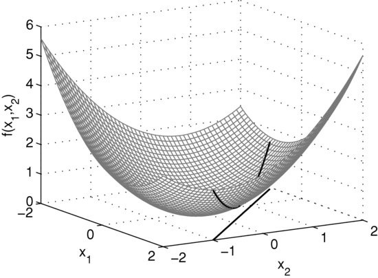
Figure 5 The Surface of a Two-Dimensional Convex Quadratic Function

Figure 6 The Contour Lines of a Two-Dimensional Convex Quadratic Function

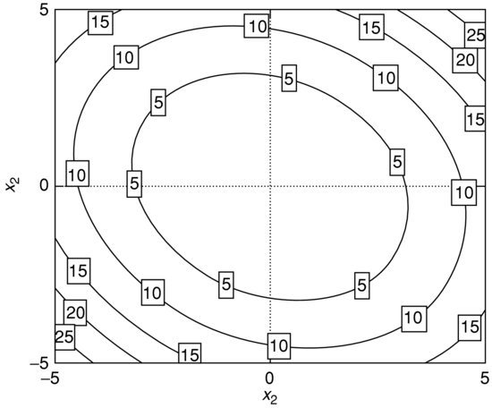
Figure 7 The Surface of a Nonconvex Two-Dimensional Quadratic Function

Figure 8 The Contour Lines of a Nonconvex Two-Dimensional Quadratic Function

Figures 5–8 illustrate the surface and contour lines of a convex and nonconvex two-dimensional quadratic function. The contour lines of the convex function are concentric ellipses and a sublevel set is represented by the points inside some ellipse. The point in Figure 8 is a saddle point. The convex quadratic function is defined by the matrix

and the nonconvex quadratic function is defined by the matrix

A property of convex functions is that the sum of convex functions is a convex function. As a result of the preceding analysis, the function

(9)

where and C is a positive semidefinite matrix, is a convex function as a sum of two convex functions. In the mean-variance efficient frontier, as formulated by Markowitz (1952), we find functions similar to (9). Let us use the properties of convex functions in order to solve the unconstrained problem of minimizing the function in (9):

This function is differentiable and we can search for the global minimum by solving the first-order conditions:

Therefore, the value of x minimizing the objective function equals

where denotes the inverse of the matrix C.

Quasi-Convex Functions

Besides convex functions, there are other classes of functions with convenient optimal properties. An example of such a class is the class of quasi-convex functions. Formally, a function is called quasi-convex if all sublevel sets defined in (7) are convex sets. Alternatively, a function f(x) is called quasi-convex if

where x1 and x2 belong to the function domain, which should be a convex set, and . A function f is called quasi-concave if is quasi-convex.

Figure 9 Example of a Two-Dimensional Quasi-Convex Function

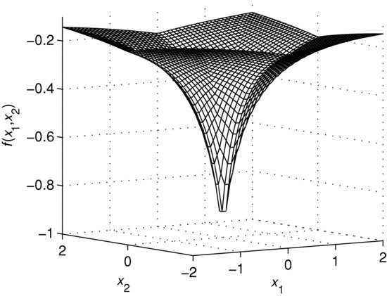
Figure 10 The Contour Lines of a Two-Dimensional Quasi-Convex Function

An illustration of a two-dimensional quasi-convex function is given in Figure 9. It shows the graph of the function and Figure 10 illustrates the contour lines. A sublevel set is represented by all points inside some contour line. From a geometric viewpoint, the sublevel sets corresponding to the plotted contour lines are convex because any of them contains the straight line connecting any two points belonging to the set. Nevertheless, the function is not convex, which becomes evident from the surface in Figure 9. It is not guaranteed that a straight line connecting any two points on the surface will remain “above” the surface.

Properties of the quasi-convex functions include:

• Any convex function is also quasi-convex. The converse is not true, which is demonstrated in Figure 10.
• In contrast to the differentiable convex functions, the first-order condition is not necessary and sufficient for optimality in the case of differentiable quasi-convex functions. (There exists a class of functions larger than the class of convex functions but smaller than the class of quasi-convex functions, for which the first-order condition is necessary and sufficient for optimality. This is the class of pseudo-convex functions. Mangasarian [2006] provides more detail on the optimal properties of pseudo-convex functions.)
• It is possible to find a sequence of convex optimization problems yielding the global minimum of a quasi-convex function. Boyd and Vandenberghe (2004) provide further details. Its main idea is to find the smallest value of c for which the corresponding sublevel set Lc is nonempty. The minimal value of c is the global minimum, which is attained in the points belonging to the sublevel set Lc.
• Suppose that is a concave function and is a convex function. Then the ratio is a quasi-concave function and the ratio is a quasi-convex function.

Quasi-convex functions arise naturally in risk management when considering optimization of performance ratios. (See Chapter in Rachev, Stoyanov, and Fabozzi [2008].)

CONSTRAINED OPTIMIZATION

In constructing optimization problems solving practical issues, it is very often the case that certain constraints need to be imposed in order for the optimal solution to make practical sense. For example, long-only portfolio optimization problems require that the portfolio weights, which represent the variables in optimization, should be nonnegative and should sum up to one. According to the notation in this chapter, this corresponds to a problem of the type

(10)

where

f(x) = the objective function
= a vector of ones,
= the sum of all components of x,
= all components of the vector are nonnegative

In problem (10), we are searching for the minimum of the objective function by varying x only in the set

(11)

which is also called the set of feasible points or the constraint set. A more compact notation, similar to the notation in the unconstrained problems, is sometimes used,

where X is defined in (11).

We distinguish between different types of optimization problems depending on the assumed properties for the objective function and the constraint set. If the constraint set contains only equalities, the problem is easier to handle analytically. In this case, the method of Lagrange multipliers is applied. For more general constraint sets, when they are formed by both equalities and inequalities, the method of Lagrange multipliers is generalized by the Karush-Kuhn-Tucker conditions (KKT conditions). Like the first-order conditions we considered in unconstrained optimization problems, none of the two approaches lead to necessary and sufficient conditions for constrained optimization problems without further assumptions. One of the most general frameworks in which the KKT conditions are necessary and sufficient is that of convex programming. We have a convex programing problem if the objective function is a convex function and the set of feasible points is a convex set. As important subcases of convex optimization, linear programming and convex quadratic programming problems are considered.

In this section, we describe first the method of Lagrange multipliers, which is often applied to special types of mean-variance optimization problems in order to obtain closed-form solutions. Then we proceed with convex programming, which is the framework for reward-risk analysis.

Lagrange Multipliers

Consider the following optimization problem in which the set of feasible points is defined by a number of equality constraints:

(12)

The functions , build up the constraint set. Note that even though the right-hand side of the equality constraints is zero in the classical formulation of the problem given in (12), this is not restrictive. If in a practical problem the right-hand side happens to be different from zero, it can be equivalently transformed; for example:

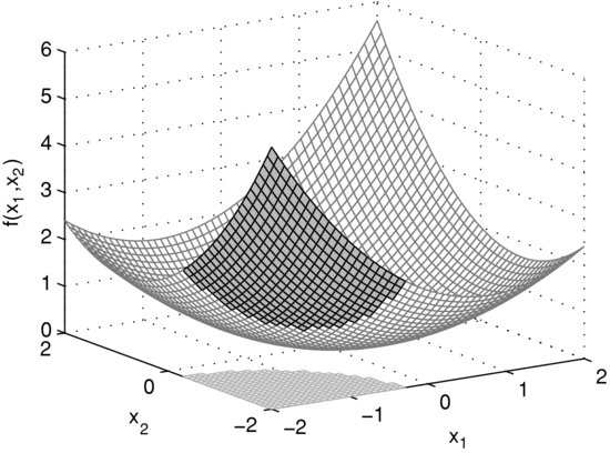
Figure 11 The Surface of a Two-Dimensional Quadratic Objective Function and the Linear Constraint

In order to illustrate the necessary condition for optimality valid for (12), let us consider the following two-dimensional example:

(13)

where the matrix is

The objective function is a quadratic function and the constraint set contains one linear equality. A mean-variance optimization problem in which short positions are allowed is very similar to (13). (See Chapter in Rachev, Stoyanov, and Fabozzi [2008].) The surface of the objective function and the constraint are shown in Figures 11 and 12. The black line on the surface shows the function values of the feasible points. Geometrically, solving problem (13) reduces to finding the lowest point of the black curve on the surface. The contour lines shown in Figure 12 imply that the feasible point yielding the minimum of the objective function is where a contour line is tangential to the line defined by the equality constraint. On the plot, the tangential contour line and the feasible points are in bold. The black dot indicates the position of the point in which the objective function attains its minimum subject to the constraints.

Figure 12 The Tangential Contour Line to the Linear Constraint

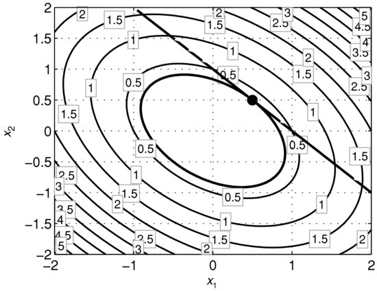
Even though the example is not general in the sense that the constraint set contains one linear rather than a nonlinear equality, the same geo-metric intuition applies in the nonlinear case. The fact that the minimum is attained where a contour line is tangential to the curve defined by the nonlinear equality constraints in mathematical language is expressed in the following way: The gradient of the objective function at the point yielding the minimum is proportional to a linear combination of the gradients of the functions defining the constraint set. Formally, this is stated as:

(14)

where , are some real numbers called Lagrange multipliers and the point is such that for all x which are feasible. Note that if there are no constraints in the problem, then (14) reduces to the first-order condition we considered in unconstrained optimization. Therefore, the system of equations behind (14) can be viewed as a generalization of the first-order condition in the unconstrained case.

The method of a Lagrange multipliers basically associates a function to the problem in (12) such that the first-order condition for unconstrained optimization for that function coincides with (14). The method of a Lagrange multiplier consists of the following steps.

1. Given the problem in (12), construct the following function:

(15)

where is the vector of Lagrange multipliers. The function is called the Lagrangian corresponding to problem (12).

2. Calculate the partial derivatives with respect to all components of x and and set them equal to zero:

(16)

Basically, the system of equations (16) corresponds to the first-order conditions for unconstrained optimization written for the Lagrangian as a function of both x and , .

3. Solve the system of equalities in (16) for x and . Note that even though we are solving the first-order condition for unconstrained optimization of , the solution of (16) is not a point of local minimum or maximum of the Lagrangian. In fact, the solution is a saddle point of the Lagrangian.

The first n equations in (16) make sure that the relationship between the gradients given in (14) is satisfied. The following k equations in (16) make sure that the points are feasible. As a result, all vectors x solving (16) are feasible and the gradient condition is satisfied at them. Therefore, the points that solve the optimization problem (12) are among the solutions of the system of equations given in (16).

This analysis suggests that the method of Lagrange multipliers provides a necessary condition for optimality. Under certain assumptions for the objective function and the functions building up the constraint set, (16) turns out to be a necessary and sufficient condition. For example, if f(x) is a convex and differentiable function and , are affine functions, then the method of Lagrange multipliers identifies the points solving (12). A function is called affine if it has the form , where a is a constant and is a vector of coefficients. All linear functions are affine. Figure 12 illustrates a convex quadratic function subject to a linear constraint. In this case, the solution point is unique.

Convex Programming

The general form of convex programming problems is

(17)

where

f(x) is a convex objective function

g1 (x), … ,gm (x) are convex functions defining the inequality constraints

h1 (x), … ,hk (x) are affine functions defining the equality constraints

Generally, without the assumptions of convexity, problem (17) is more involved than (12) because besides the equality constraints, there are inequality constraints. The KKT condition, generalizing the method of Lagrange multipliers, is only a necessary condition for optimality in this case. However, adding the assumption of convexity makes the KKT condition necessary and sufficient.

Note that, similar to problem (12), the fact that the right-hand side of all constraints is zero is nonrestrictive. The limits can be arbitrary real numbers.

Figure 13 The Surface of a Two-Dimensional Convex Quadratic Function and a Convex Quadratic Constraint

Consider the following two-dimensional optimization problem

(18)

in which

The objective function is a two-dimensional convex quadratic function and the function in the constraint set is also a convex quadratic function. In fact, the boundary of the feasible set is a circle with a radius of centered at the point with coordinates . Figures 13 and 14 show the surface of the objective function and the set of feasible points. The shaded part on the surface indicates the function values of all feasible points. In fact, solving problem (18) reduces to finding the lowest point on the shaded part of the surface. Figure 14 shows the contour lines of the objective function together with the feasible set, which is in gray. Geometrically, the point in the feasible set yielding the minimum of the objective function is positioned where a contour line only touches the constraint set. The position of this point is marked with a black dot and the tangential contour line is given in bold.

Figure 14 The Tangential Contour Line to the Feasible Set Defined by a Convex Quadratic Constraint

Note that the solution points of problems of the type (18) can happen to be not on the boundary of the feasible set but in the interior. For example, suppose that the radius of the circle defining the boundary of the feasible set in (18) is a larger number such that the point is inside the feasible set. Then, the point is the solution to problem (18) because at this point the objective function attains its global minimum.

In the two-dimensional case, when we can visualize the optimization problem, geometric reasoning guides us to finding the optimal solution point. In a higher dimensional space, plots cannot be produced and we rely on the analytic method behind the KKT conditions. The KKT conditions corresponding to the convex programming problem (17) are the following:

(19)

A point x0 such that satisfies (19) is the solution to problem (17). Note that if there are no inequality constraints, then the KKT conditions reduce to (16) in the method of Lagrange multipliers. Therefore, the KKT conditions generalize the method of Lagrange multipliers.

The gradient condition in (19) has the same interpretation as the gradient condition in the method of Lagrange multipliers. The set of constraints

guarantee that a point satisfying (19) is feasible. The next conditions

are called complementary slackness conditions. If an inequality constraint is satisfied as a strict inequality, then the corresponding multiplier turns into zero according to the complementary slackness conditions. In this case, the corresponding gradient has no significance in the gradient condition. This reflects the fact that the gradient condition concerns only the constraints satisfied as equalities at the solution point.

Important special cases of convex programming problems include linear programming problems and convex quadratic programming problems, which we consider in the remaining part of this section.

Linear Programming

Optimization problems are said to be linear programming problems if the objective function is a linear function and the feasible set is defined by linear equalities and inequalities. Since all functions are linear, they are also convex, which means that linear programming problems are also convex problems. The definition of linear programming problems in standard form is the following:

(20)

where A is an matrix of coefficients, is a vector of objective function coefficients, and is a vector of real numbers. As a result, the constraint set contains m inequalities defined by linear functions. The feasible points defined by means of linear equalities and inequalities are also said to form a polyhedral set. In practice, before solving a linear programming problem, it is usually first reformulated in the standard form given in (20).

Figure 15 The Surface of a Linear Function and a Polyhedral Feasible Set

Figure 16 The Bottom Plot Shows the Tangential Contour Line to the Polyhedral Feasible Set

Figures 15 and 16 show an example of a two-dimensional linear programming problem which is not in standard form as the two variables may become negative. Figure 15 contains the surface of the objective function, which is a plane in this case, and the polyhedral set of feasible points. The shaded area on the surface corresponds to the points in the feasible set. Solving problem (20) reduces to finding the lowest point in the shaded area on the surface. Figure 16 shows the feasible set together with the contour lines of the objective function. The contour lines are parallel straight lines because the objective function is linear. The point in which the objective function attains its minimum is marked with a black dot.

A general result in linear programming is that, on condition that the problem is bounded, the solution is always at the boundary of the feasible set and, more precisely, at a vertex of the polyhedron. Problem (20) may become unbounded if the polyhedral set is unbounded and there are feasible points such that the objective function can decrease indefinitely. We can summarize that, generally, due to the simple structure of (20), there are three possibilities:

From computational viewpoint, the polyhedral set has a finite number of vertices and an algorithm can be devised with the goal of finding a vertex solving the optimization problem in a finite number of steps. This is the basic idea behind the simplex method, which is an efficient numerical approach to solving linear programming problems. Besides the simplex algorithm, there are other, more contemporary methods, such as the interior point method.

Quadratic Programming

Besides linear programming, another class of problems with simple structure is the class of quadratic programming problems. It contains optimization problems with a quadratic objective function and linear equalities and inequalities in the constraint set:

(21)

where

c = (c1, …, cn) is a vector of coefficients defining the linear part of the objective function

H={hij}i,j = 1n is an $n imes n$ matrix defining the quadratic part of the objective

A = {aij} is a k × n matrix defining k linear inequalities in the constraint set

b = (b1, …, bk) is a vector of real numbers defining the right-hand side of the linear inequalities

In optimal portfolio theory, mean-variance optimization problems in which portfolio variance is in the objective function are quadratic programming problems.

From the point of view of optimization theory, problem (21) is a convex optimization problem if the matrix defining the quadratic part of the objective function is positive semidefinite. In this case, the KKT conditions can be applied to solve it.

KEY POINTS

REFERENCES

Boyd, S., and Vandenberghe, L. (2004). Convex Optimization. Cambridge: Cambridge University Press.

Markowitz, H. M. (1952). Portfolio selection. Journal of Finance 7, 1: 77–91.

Mangasarian, O. (2006). Pseudo-convex functions. In W. Ziemba and G. Vickson (eds.), Stochastic Optimization Models in Finance (pp. 23–32), Singapore: World Scientific Publishing.

Rachev, Z. T., Stoyanov, S., and Fabozzi, F. J. (2008). Advanced Stochastic Models, Risk Assessment and Portfolio Optimization: The Ideal Risk, Uncertainty and Performance Measures. Hoboken, NJ: John Wiley & Sons.

Rockafellar, R. T. (1997). Convex Analysis. Princeton, NJ: Princeton University Press, Landmarks in Mathematics.

Ruszczynski, A. (2006). Nonlinear Optimization. Princeton, NJ: Princeton University Press.