
Asset Allocation and Portfolio Construction Techniques in Designing the Performance-Seeking Portfolio
Management is justified as an industry by the capacity of adding value through the design of investment solutions that match investors’ needs. For more than 50 years, the industry has in fact mostly focused on security selection decisions as a single source of added value. This sole focus has somewhat distracted the industry from another key source of added value, namely portfolio construction and asset allocation decisions. In the face of recent crises, and given the intrinsic difficulty in delivering added value through security selection decisions only, the relevance of the old paradigm has been questioned with heightened intensity, and a new paradigm is starting to emerge.
Academic research has provided very useful guidance with respect to how asset allocation and portfolio construction decisions should be analyzed so as to best improve investors’ welfare. In a nutshell, the “fund separation theorems” that lie at the core of modern portfolio theory advocate a separate management of performance and risk control objectives. In the context of asset allocation decisions with consumption/liability objectives, it can be shown that the suitable expression of the fund separation theorem provides rational support for liability-driven investment (LDI) techniques that have recently been promoted by a number of investment banks and asset management firms. These solutions involve on the one hand the design of a customized liability-hedging portfolio (LHP), the sole purpose of which is to hedge away as effectively as possible the impact of unexpected changes in risk factors affecting liability values (most notably interest rate and inflation risks), and on the other hand the design of a performance-seeking portfolio (PSP), whose raison d’être is to provide investors with an optimal risk-return trade-off.
One of the implications of this LDI paradigm is that one should distinguish two different levels of asset allocation decisions: allocation decisions involved in the design of the performance-seeking or the liability-hedging portfolio (design of better building blocks, or BBBs), and asset allocation decisions involved in the optimal split between the PSP and the LHP (designed of advanced asset allocation decisions, or AAAs). We address the question of better building blocks in detail in this entry and provide some thoughts on integrating these building blocks in asset allocation. More specifically, we mainly focus here on how to construct efficient performance-seeking portfolios.
In this entry we provide an overview of the key conceptual challenges involved in asset allocation and portfolio construction in designing the performance-seeking portfolio. We begin by presenting the fundamental principle of the maximization of risk/reward efficiency and then deal with estimation of risk parameters and expected return parameters. The empirical results of optimal portfolio construction modeling are presented. We also provide a brief discussion on integrating such properly designed building blocks in the overall PSP at the asset allocation level.
THE TANGENCY PORTFOLIO AS THE RATIONALE BEHIND SHARPE RATIO MAXIMIZATION
Modern portfolio theory provides some useful guidance with respect to the optimal design of a PSP that would best suit investors’ needs. More precisely, the prescription is that the PSP should be obtained as the result of a portfolio optimization procedure aiming at generating the highest risk-reward ratio.
Portfolio optimization is a straightforward procedure, at least in principle. In a mean-variance setting, for example, the prescription consists of generating a maximum Sharpe ratio (MSR) portfolio based on expected return, volatility, and pairwise correlation parameters for all assets to be included in the portfolio, a procedure that can even be handled analytically in the absence of portfolio constraints.
More precisely, consider a simple mean-variance problem:
![]()
Here, the control variable is a vector w of optimal weight allocated to various risky assets, μp denotes the portfolio expected return, and σp denotes the portfolio volatility. We further assume that the investor is facing the following investment opportunity set: a riskless bond paying the risk-free rate r, and a set of N risky assets with expected return vector μ (of size N) and covariance matrix Σ (of size NxN), all assumed constant so far.
With these notations, the portfolio expected return and volatility are respectively given by:
![]()
In this context, it is straightforward to show by standard arguments that the only efficient portfolio composed with risky assets is the maximum Sharpe ratio portfolio, also known as the tangency portfolio.1
Finally, the Sharpe ratio reads (where we further denote by e vector of ones of size N):
![]()
And the optimal portfolio is given by:
This is a two-fund separation theorem, which gives the allocation to the MSR performance-seeking portfolio (PSP), with the rest invested in cash, as well as the composition of the MSR performance-seeking portfolio.
In practice, investors end up holding more or less imperfect proxies for the truly optimal performance-seeking portfolio, if only because of the presence of parameter uncertainty, which makes it impossible to obtain a perfect estimate for the maximum Sharpe ratio portfolio. Denoting by λ the Sharpe ratio of the (generally inefficient) PSP actually held by the investor, and by σ its volatility, we obtain the following optimal allocation strategy:
(2) ![]()
Hence the allocation to the performance-seeking portfolio is a function of two objective parameters, the PSP volatility and the PSP Sharpe ratio, and one subjective parameter, the investor’s risk aversion. The optimal allocation to the PSP is inversely proportional to the investor’s risk aversion. If risk aversion goes to infinity, the investor holds the risk-free asset only, as should be expected. For finite risk-aversion levels, the allocation to the PSP is inversely proportional to the PSP volatility, and it is proportional to the PSP Sharpe ratio. As a result, if the Sharpe ratio of the PSP is increased, one can invest more in risky assets. Hence, portfolio construction modeling is not only about risk reduction; it is also about performance enhancement through a better spending of investors’ risk budgets.
The expression (1) is useful because it provides in principle a straightforward expression for the optimal portfolio starting from a set of N risky assets. In the presence of a realistically large number N of securities, the curse of dimensionality, however, makes it practically impossible for investors to implement such direct one-step portfolio optimization decisions involving all individual components of the asset mix. The standard alternative approach widely adopted in investment practice consists instead in first grouping individual securities in various asset classes according to various dimensions, for example, country, sector, and/or style within the equity universe, or country, maturity, and credit rating within the bond universe, and subsequently generating the optimal portfolio through a two-stage process. On the one hand, investable proxies are generated for maximum Sharpe ratio (MSR) portfolios within each asset class in the investment universe. We call this step, which is typically delegated to professional money managers, the portfolio construction step. On the other hand, when the MSR proxies are obtained for each asset class, an optimal allocation to the various asset classes is eventually generated so as to generate the maximum Sharpe ratio at the global portfolio level. This step is called the asset allocation step, and it is typically handled by a centralized decision maker (e.g., a pension fund CIO) with or without the help of specialized consultants, as opposed to being delegated to decentralized asset managers. In this entry, the discussion focuses on the first step, and we provide some concluding remarks on its relation to the second step at the end of this entry.
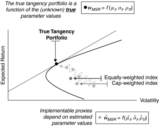
For the definition of building blocks for asset allocation, in the absence of active views, the default option consists of using market cap weighted indexes as proxies for the asset class MSR portfolio. Academic research, however, has found that such market cap indexes were likely to be severely inefficient portfolios.2 In a nutshell, market cap weighted indexes are not good choices as investment benchmarks because they are poorly diversified portfolios. In fact, cap-weighting tends to lead to exceedingly high concentration in relatively few stocks. As a consequence of their lack of diversification, cap weighted indexes have been empirically found to be severely inefficient portfolios, which do not provide investors with the fair reward given the risk taken. As a result of their poor diversification, they have been found to be dominated by equally weighted benchmarks,3 which are naïvely diversified portfolios that are optimal if and only if all securities have identical expected return, volatilities, and all pairs of correlations are identical.
In what follows, we analyze in some detail a number of alternatives based on practical implementation of modern portfolio theory that have been suggested to generate more efficient proxies for the MSR portfolio in the equity investment universe. (See Figure 1.)
Figure 1 Inefficiency of Cap-Weighted Benchmarks, and the Quest for an Efficient Proxy for the True Tangency Portfolio
Modern portfolio theory was born with the efficient frontier analysis of Markowitz (1952). Unfortunately, early applications of the technique, based on naïve estimates of the input parameters, have been found of little use because they lead to nonsensible portfolio allocations.
In a first section, we explain how to help bridge the gap between portfolio theory and portfolio construction by showing how to generate enhanced parameter estimates so as to improve the quality of the portfolio optimization outputs (optimal portfolio weights). We first focus on enhanced covariance parameter estimates and explain how to meet the main challenge of sample risk reduction.4 Against this backdrop, we present the state-of-the art methodologies for reducing the problem dimensionality and estimating the covariance matrix with multifactor models. We then turn to expected return estimation. We argue that statistical methodologies are not likely to generate any robust expected return estimates, which suggests that economic models such as the single-factor CAPM and the multifactor APT should instead be used for expected return estimation. Finally, we also present evidence that proxies for expected return estimates should not only include systematic risk measures, but they should also incorporate idiosyncratic risk measures as well as downside risk measures.
ROBUST ESTIMATORS FOR COVARIANCE PARAMETERS
In practice, success in the implementation of a theoretical model relies not only upon its conceptual grounds but also on the reliability of the inputs of the model. In the case of mean-variance (MV) optimization the results will highly depend on the quality of the parameter estimates: the covariance matrix and the expected returns of assets.
Several improved estimates for the covariance matrix have been proposed, including most notably the factor-based approach suggested by Sharpe (1963), the constant correlation approach suggested by Elton and Gruber (1973), and the statistical shrinkage approach suggested by Ledoit and Wolf (2004). In addition, Jagannathan and Ma (2003) find that imposing (non–short selling) constraints on the weights in the optimization program improves the risk-adjusted out-of-sample performance in a manner that is similar to some of the aforementioned improved covariance matrix estimators.
In these papers, the authors have focused on testing the out-of-sample performance of global minimum variance (GMV) portfolios, as opposed to the MSR portfolios (also known as tangency portfolios), given that there is a consensus around the fact that purely statistical estimates of expected returns are not robust enough to be used. (This is discussed later in this entry.)
The key problem in covariance matrix estimation is the curse of dimensionality; when a large number of stocks are considered, the number of parameters to estimate grows exponentially, where the majority of them are pairwise correlations.
Therefore, at the estimation stage, the challenge is to reduce the number of factors that come into play. In general, a multifactor model decomposes the (excess) return (in excess to the risk-free asset) of an asset into its expected rewards for exposition to the “true” risk factors as follows:
![]()
or in matrix form for all N assets:
![]()
where βt is an N × K matrix containing the sensitivities of each asset i with respect to the corresponding j-th factor movements; rt is the vector of the N assets’ (excess) returns, Ft a vector containing the K risk factors’ (excess) returns, and εt the N × 1 vector containing the zero mean uncorrelated residuals εit.The covariance matrix for the asset returns implied by a factor model is given by:
![]()
where ΣF is the K × K covariance matrix of the risk factors and Σε an N × N covariance matrix of the residuals corresponding to each asset.
While the factor-based estimator is expected to allow for a reasonable trade-off between sample risk and model risk, there still remains, however, the problem of choosing the “right” factor model. One popular approach aims at relying as little as possible on strong theoretical assumptions by using principal components analysis (PCA) to determine the underlying risk factors from the data. The PCA method is based on a spectral decomposition of the sample covariance matrix, and its goal is to explain covariance structures using only a few linear combinations of the original stochastic variables, which will constitute the set of (unobservable) factors.
Bengtsson and Holst (2002) and Fujiwara et al. (2006) motivate the use of PCA in a similar way, extracting principal components in order to estimate expected correlation within MV portfolio optimization. Fujiwara et al. (2006) find that the realized risk-return of portfolios based on the PCA method outperforms the single-index-based one and that the optimization gives a practically reasonable asset allocation. Overall, the main strength of the PCA approach at this stage is that it allows “the data to talk” and has them tell the financial modeler what the underlying risk factors are that govern most of the variability of the assets at each point in time. This strongly contrasts with having to rely on the assumption that a particular factor model is the true pricing model and reduces the specification risk embedded in the factor-based approach while keeping the sample risk reduction.
The question of determining the appropriate number of factors to structure the correlation matrix is critical for the risk estimation when using PCA as a factor model. Several options have been proposed to answer this question, some of them with more theoretical grounds than others.
As a final note, we need to recognize that the discussion is so far cast in a mean-variance setting, which can in principle only be rationalized for normally distributed asset returns. In the presence of non-normally distributed asset returns, optimal portfolio selection techniques require estimates for variance-covariance parameters, along with estimates for higher-order moments and comoments of the return distribution. This is a formidable challenge that severely exacerbates the dimensionality problem already present with mean-variance analysis. In a recent paper, Martellini and Ziemann (2010) extend the existing literature, which has mostly focused on the covariance matrix, by introducing improved estimators for the coskewness and cokurtosis parameters. On the one hand, they find that the use of these enhanced estimates generates a significant improvement in investors’ welfare. On the other hand, they find that also that when the number of constituents in the portfolios is large (e.g., exceeding 20), the increase in sample risk related to the need to estimate higher-order comoments by far outweighs the benefits related to considering a more general portfolio optimization procedure. In the end, when portfolio optimization is performed on the basis of a large number of individual securities, it appears that maximizing the portfolio Sharpe ratio leads to a better out-of-sample return-to-VaR ratio or return-to-CVaR ratio compared to a procedure focusing on maximizing the return-to-VaR ratio or the return-to-CVaR ratio, a result that holds true even if improved estimators are used for higher-order comoments.
ROBUST ESTIMATORS FOR EXPECTED RETURNS
While it appears that risk parameters can be estimated with a fair degree of accuracy, it has been shown (Merton, 1980) that expected returns are difficult to obtain with a reasonable estimation error. What makes the problem worse is that optimization techniques are very sensitive to differences in expected returns, so that portfolio optimizers typically allocate the largest fraction of capital to the asset class for which estimation error in the expected returns is the largest.5
In the face of the difficulty of using sample-based expected return estimates in a portfolio optimization context, a reasonable alternative consists in using some risk estimate as a proxy for excess expected returns.6 This approach is based on the most basic principle in finance; that is, the natural relationship between risk and reward. In fact, standard asset pricing theories such as the arbitrage pricing theory as proposed by Ross (1976) imply that expected returns should be positively related to systematic volatility, such as measured through a factor model that summarizes individual stock return exposure with respect to a number of rewarded risk factors.
More recently, a series of papers have focused on the explanatory power of idiosyncratic, as opposed to systematic, risk for the cross section of expected returns. In particular, Malkiel and Xu (2006), extending an insight from Merton (1987), show that an inability to hold the market portfolio, whatever the cause, will force investors to care about total risk to some degree in addition to market risk so that firms with larger firm-specific variances require higher average returns to compensate investors for holding imperfectly diversified portfolios.7 That stocks with high idiosyncratic risk earn higher returns has also been confirmed in a number of recent empirical studies, including in particular Tinic and West (1986) as well as Malkiel and Xu (1997, 2006).
Taken together, these findings suggest that total risk, a model-free quantity given by the sum of systematic and specific risk, should be positively related to expected return. Most commonly, total risk is the volatility of a stock’s returns. Martellini (2008) has investigated the portfolio implications of these findings and has found that tangency portfolios constructed on the assumption that the cross-section of excess expected returns could be approximated by the cross-section of volatility posted better out-of-sample risk-adjusted performance than their market-cap-weighted counterparts.
More generally, recent research suggests that the cross-section of expected returns might be best explained by risk indicators taking into account higher-order moments. Theoretical models have shown that, in exchange for higher skewness and lower kurtosis of returns, investors are willing to accept expected returns lower (and with volatility higher) than those of the mean-variance benchmark.8 More specifically, skewness and kurtosis in individual stock returns (as opposed to the skewness and kurtosis of aggregate portfolios) have been shown to matter in several papers. High skewness is associated with lower expected returns in Barberis and Huang (2004), Brunnermeier, Gollier, and Parker (2005), and Mitton and Vorkink (2007). The intuition behind this result is that investors like to hold positively skewed portfolios. The highest skewness is achieved by concentrating portfolios in a small number of stocks that themselves have positively skewed returns. Thus investors tend to be underdiversified and drive up the price of stocks with high positive skewness, which in turn reduces their future expected returns. Stocks with negative skewness are relatively unattractive and thus have low prices and high returns. The preference for kurtosis is in the sense that investors like low kurtosis and thus expected returns should be positively related to kurtosis. Boyer, Mitton, and Vorkink (2010) and Conrad, Dittmar and Ghysels (2008) provide empirical evidence that individual stocks’ skewness and kurtosis is indeed related to future returns. An alternative to direct consideration of the higher moments of returns is to use a risk measure that aggregates the different dimensions of risk. In this line, Bali and Cakici (2004) show that future returns on stocks are positively related to their value-at-risk and Estrada (2000) and Chen, Chen, and Chen (2009) show that there is a relationship between downside risk and expected returns.
IMPLICATIONS FOR BENCHMARK PORTFOLIO CONSTRUCTION
Once careful estimates for risk and return parameters have been obtained, one may then design efficient proxies for an asset class benchmark with an attractive risk-return profile. For example, Amenc et al. (2011) find that efficient equity benchmarks designed on the basis of robust estimates for risk and expected return parameters substantially outperform in terms of risk-adjusted performance market cap weighted indexes that are often used as default options for investment benchmarks in spite of their well-documented lack of efficiency.9
Table 1, borrowed from Amenc et al. (2011), shows summary performance statistics for an efficient index constructed according to the aforementioned principles. For the average return, volatility, and the Sharpe ratio, we report differences with respect to cap-weighting and assess whether this difference is statistically significant.
Table 1 Risk and Return Characteristics for the Efficient Index
Table 1 shows that the efficient weighting of index constituents leads to higher average returns, lower volatility, and a higher Sharpe ratio. All these differences are statistically significant at the 10% level, whereas the difference in Sharpe ratios is significant even at the 0.1% level. Given the data, it is highly unlikely that the unobservable true performance of efficient weighting was not different from that of capitalization weighting. Economically, the performance difference is pronounced, as the Sharpe ratio increases by about 70%.
ASSET ALLOCATION MODELING: PUTTING THE EFFICIENT BUILDING BLOCKS TOGETHER
After efficient benchmarks have been designed for various asset classes, these building blocks can be assembled in a second step, the asset allocation step, to build a well-designed multiclass performance-seeking portfolio.
While the methods we have discussed so far can in principle be applied in both contexts, a number of key differences should be emphasized.
In the asset allocation context, the number of constituents is small, and using time- and state-dependent covariance matrix estimates becomes reasonable, while they do not necessarily improve the situation in portfolio construction contexts when the number of constituents is large. Similarly, while it is not feasible in general, as explained above, to perform portfolio optimization with higher-order moments in a portfolio construction context where the number of constituents is typically large, it is reasonable to go beyond mean-variance analysis in an asset allocation context where the number of constituents is limited.
Furthermore, in an asset allocation context, the universe is not homogenous, which has implications for expected returns and covariance estimation. In terms of a covariance matrix, it will not prove easy to obtain a universal factor model for the whole investment universe. In this context, it is arguably better to use statistical shrinkage toward, say, the constant correlation model, as opposed to using a factor model approach.10
KEY POINTS
- Modern portfolio theory advocates the separation of the management of performance and risk control objectives. In the context of asset allocation decisions, the fund separation theorem provides rational support for liability-driven investment techniques whose solutions involve the design of a customized liability-hedging portfolio and the design of a performance-seeking portfolio.
- The sole purpose of the liability-hedging portfolio is to hedge away as effectively as possible the impact of unexpected changes in risk factors affecting liability values (most notably interest rate and inflation risks); the purpose of the performance-seeking portfolio is to provide investors with an optimal risk-return trade-off.
- An implication of the liability-driven investment paradigm is that one should distinguish two different levels of asset allocation decisions: (1) decisions involved in the design of the performance-seeking or the liability-hedging portfolio (design of better building blocks), and (2) decisions involved in the optimal split between the performance-seeking portfolio and liability-hedging portfolio (designed of advanced asset allocation decisions).
- Although modern portfolio theory provides some useful guidance with respect to the optimal design of performance-seeking portfolios that would best suit investors’ needs, in practice, investors end up holding more or less imperfect proxies for the truly optimal performance-seeking portfolio, if only because of the presence of parameter uncertainty, which makes it impossible to obtain a perfect estimate for the maximum Sharpe ratio portfolio.
- The allocation to the performance-seeking portfolio is a function of two objective parameters, the PSP volatility and the PSP Sharpe ratio, and one subjective parameter, the investor’s risk aversion. The optimal allocation to the PSP is inversely proportional to the investor’s risk aversion.
- In practice, the success in the implementation of a theoretical model relies not only upon its conceptual grounds but also on the reliability of the inputs of the model. In the case of mean-variance optimization the results will highly depend on the quality of the parameter estimates: the covariance matrix and the expected returns of assets.
- Several improved estimates for the covariance matrix have been proposed: the factor-based approach, constant correlation approach, and statistical shrinkage approach.
- The key problem in covariance matrix estimation is the curse of dimensionality. Consequently, at the estimation stage, the challenge is to reduce the number of factors that come into play. In general, a multifactor model decomposes the (excess) return (in excess to the risk-free asset) of an asset into its expected rewards for exposition to the “true” risk factors.
- The problem of choosing the right factor model still remains. The statistical technique of principal components analysis is commonly used to determine the underlying risk factors from the data.
- While it appears that risk parameters can be estimated with a fair degree of accuracy, it has been shown that expected returns are difficult to obtain with a reasonable estimation error. What makes the problem worse is that optimization techniques are very sensitive to differences in expected returns, so that portfolio optimizers typically allocate the largest fraction of capital to the asset class for which estimation error in the expected returns is the largest. In the face of the difficulty of using sample-based expected return estimates in a portfolio optimization context, a reasonable alternative consists in using some risk estimate as a proxy for excess expected returns.
- Research suggests that the cross-section of expected returns might be best explained by risk indicators taking into account higher-order moments. Theoretical models have shown that, in exchange for higher skewness and lower kurtosis of returns, investors are willing to accept expected returns lower (and volatility higher) than those of the mean-variance benchmark.
- Once careful estimates for risk and return parameters have been obtained, one may then design efficient proxies for an asset class benchmark with an attractive risk-return profile. After efficient benchmarks have been designed for various asset classes, these building blocks can be assembled in a second step, the asset allocation step, to build a well-designed multiclass performance- seeking portfolio.
NOTES
1. For more details, see Appendix A.1 in Amenc, Goltz, Martellini, and Mihau (2011).
2. See, for example, Haugen and Baker (1991), Grinold (1992), or Amenc, Goltz, and Le Sourd (2006).
3. De Miguel et al. (2009).
4. Another key challenge is the presence of nonstationary risk parameters, which can be accounted for with conditional factor models capturing time-dependencies (e.g., GARCH-type models) and state-dependencies (e.g., Markov regime switching models) in risk parameter estimates.
5. See Britten-Jones (1999) or Michaud (1998).
6. This discussion focuses on estimating the fair neutral reward for holding risky assets. If one has access to active views on expected returns, one may use a disciplined approach (e.g., the Black-Litterman model) to combine the active views with the neutral estimates.
7. See also Barberis and Huang (2001) for a similar conclusion from a behavioral perspective.
8. See Rubinstein (1973) and Kraus and Litzenberger (1976).
9. See, for example, Haugen and Baker (1991) and Grinold (1992).
10. See Ledoit and Wolf (2003, 2004).
REFERENCES
Amenc, N., Goltz, F., and Le Sourd, V. (2006). Assessing the quality of stock market indices. EDHEC-Risk Institute Publication (September).
Amenc, N., Goltz, F., Martellini, L., and Milhau, V. (2011). Asset allocation and portfolio construction. In F. J. Fabozzi and H. M. Markowitz (Eds.), The Theory and Practice of Investment Management: Second Edition. Hoboken, NJ: John Wiley & Sons.
Amenc, N., Goltz, F., Martellini, L., and Retkowsky, P. Efficient indexation: An alternative to cap-weighted indices. Journal of Investment Management, forthcoming.
Bali, T., and Cakici, N. (2004). Value at risk and expected stock returns. Financial Analysts Journal 60, 2 (March/April): 57–73.
Barberis, N., and Huang, M. (2004). Stock as lotteries: The implication of probability weighting for security prices. Working paper (Stanford and Yale University).
Barberis, N., and Huang, M. (2001). Mental accounting, loss aversion and individual stock returns. Journal of Finance 56, 4 (August): 1247–1292.
Bengtsson, C., and Holst, J. (2002). On portfolio selection: Improved covariance matrix estimation for Swedish asset returns. Working paper (Lund University and Lund Institute of Technology).
Boyer, B., Mitton, T., and Vorkink, K. (2010). Expected idiosyncratic skewness. Review of Financial Studies 23, 1 (January): 169–202.
Britten-Jones, M. (1999). The sampling error in estimates of mean-variance efficient portfolio weights. Journal of Finance 54, 2 (April): 655–671.
Brunnermeier, M. K., Gollier, C., and Parker, J. (2007). Optimal beliefs, asset prices, and the preference for skewed returns. American Economic Review 97, 2 (May): 159–165.
Chen, D. H., Chen, C. D., and Chen, J. (2009). Downside risk measures and equity returns in the NYSE. Applied Economics 41, 8 (March): 1055–1070.
Conrad, J., Dittmar, R. F., and Ghysels, E. (2008). Ex ante skewness and expected stock returns. Working paper (University of North Carolina at Chapel Hill).
De Miguel, V., Garlappi, L., and Uppal, R. (2009). Optimal versus naive diversification: How inefficient is the 1/N portfolio strategy? Review of Financial Studies 22, 5: 1915–1953.
Elton, E., and Gruber, M. (1973). Estimating the dependence structure of share prices: Implications for portfolio selection. Journal of Finance 28, 5 (December): 1203–1232.
Estrada, J. (2000). The cost of equity in emerging markets: A downside risk approach. Emerging Markets Quarterly 4, 2 (fall): 19–30.
Fujiwara, Y., Souma, W., Murasato, H., and Yoon, H. (2006). Application of PCA and random matrix theory to passive fund management. In Hideki Takayasu (ed.), Practical Fruits of Econophysics. Tokyo: Springer, 226–230.
Grinold, R. C. (1992). Are benchmark portfolios efficient? Journal of Portfolio Management 19, 1 (autumn): 34–40.
Haugen, R. A., and Baker, N. L. (1991). The efficient market inefficiency of capitalisation-weighted stock portfolios. Journal of Portfolio Management 17, 3 (spring): 35–40.
Jagannathan, R., and Ma, T. (2003). Risk reduction in large portfolios: Why imposing the wrong constraints helps. Journal of Finance 58, 4 (August): 1651–1684.
Krauz, A., and Litzenberger, R. H. (1976). Skewness preference and the valuation of risk assets. Journal of Finance 31, 4 (September): 1085–1100.
Ledoit, O., and Wolf, M. (2004). Honey, I shrunk the sample covariance matrix. Journal of Portfolio Management 30, 4 (summer): 110–119.
Ledoit, O., and Wolf, M. (2003). Improved estimation of the covariance matrix of stock returns with an application to portfolio selection. Journal of Empirical Finance 10, 5 (December): 603–621.
Malkiel, B., and Xu, Y. (2006). Idiosyncratic risk and security returns. Working paper (University of Texas at Dallas).
Malkiel, B., and Xu, Y. (1997). Risk and return revisited. Journal of Portfolio Management 23, 3 (spring): 9–14.
Markowitz, H. (1952). Portfolio selection. Journal of Finance 7, 1 (March): 77–91.
Martellini, L. (2008). Towards the design of better equity benchmarks: Rehabilitating the tangency portfolio from modern portfolio theory. Journal of Portfolio Management 34, 4 (summer): 34–41.
Martellini, L., and Ziemann, V. (2010). Improved estimates of higher-order comoments and implications for portfolio selection. Review of Financial Studies 23, 4 (April): 1467–1502.
Merton, R. C. (1987). A simple model of capital market equilibrium with incomplete information. Journal of Finance 42, 3 (July): 483–510.
Merton, R. C. (1980). On estimating the expected return on the market: An exploratory investigation. Journal of Financial Economics 8, 4 (December): 323–361.
Michaud, R. (1998). Efficient Asset Management: A Practical Guide to Stock Portfolio Optimization and Asset Allocation. Boston, MA: Harvard Business School Press.
Mitton, T., and Vorkink, K. (2007). Equilibrium underdiversification and the preference for skewness. Review of Financial Studies 20, 4 (July): 1255–1288.
Ross, S. A. (1976). The arbitrage theory of capital asset pricing. Journal of Economic Theory 13, 3 (December): 341–360.
Rubinstein, M. E. (1973). The fundamental theorem of parameter-preference security valuation. Journal of Financial and Quantitative Analysis 8, 1 (January): 61–69.
Sharpe, W. F. (1963). A simplified model for portfolio analysis. Management Science 9, 2 (January): 277–293.
Tinic, S., and West, R. (1986). Risk, return and equilibrium: A revisit. Journal of Political Economy 94, 1 (February): 126–147.