
Applying Cointegration to Problems in Finance
The long-term relationships among economic variables, such as short-term versus long-term interest rates, or stock prices versus dividends, have long interested finance practitioners. For certain types of trends, multiple regression analysis needs modification to uncover these relationships. A trend represents a long-term movement in the variable. One type of trend, a deterministic trend, has a straightforward solution. Since a deterministic trend is a function of time, we merely include this time function in the regression. For example, if the variables are increasing or decreasing as a linear function of time, we may simply include time as a variable in the regression equation. The issue becomes more complex when the trend is stochastic. A stochastic trend is defined (Stock and Watson, 2003) as “a persistent but random long-term movement of the variable over time.” Thus a variable with a stochastic trend may exhibit prolonged long-run increases followed by prolonged long-run declines and perhaps another period of long-term increases.
Most financial theorists believe stochastic trends better describe the behavior of financial variables than deterministic trends. For example, if stock prices are rising, there is no reason to believe they will continue to do so in the future. Or, even if they continue to increase in the future, they may not do so at the same rate as in the past. This is because stock prices are driven by a variety of economic factors and the impact of these factors may change over time. One way of capturing these common stochastic trends is by using an econometric technique usually referred to as cointegration.
In this entry, we explain the concept of cointegration. There are two major ways of testing for cointegration. We outline both econometric methods and the underlying theory for each method. We illustrate the first technique with an example of the first type of cointegration problem, testing market efficiency. Specifically, we examine the present value model of stock prices. We illustrate the second technique with an example of the second type of cointegration problem, examining market linkages. In particular, we test the linkage and the dynamic interactions among stock market indexes of three European countries. Finally, we also use cointegration to test for the presence of an asset price bubble. Specifically, we test for the possibility of bubbles in the real estate markets.
STATIONARY AND NONSTATIONARY VARIABLES AND COINTEGRATION
The presence of stochastic trends may lead a researcher to conclude that two economic variables are related over time when in fact they are not. This problem is referred to as spurious regression. For example, during the 1980s the U.S. stock market and the Japanese stock market were both rising. An ordinary least squares (OLS) regression of the U.S. Morgan Stanley Stock Index on the Japanese Morgan Stanley Stock Index (USD) for the time period 1980–1990 using monthly data yields
The t-statistic on the slope coefficient (26.51) is quite large, indicating a strong positive relationship between the two stock markets. This strong relationship is reinforced with a very high R-square value. However, estimating the same regression over a different time period, 1990–2007, reveals
This regression equation suggests there is a strong negative relationship between the two stock market indexes. Although the t-statistic on the slope coefficient (2.80) is large, the low R-square value suggests that the relationship is rather weak.
The reason behind these contradictory results is the presence of stochastic trends in both series. During the first time span, these stochastic trends were aligned, but not during the latter time span. Since different economic forces influence the stochastic trends and these forces change over time, during some periods they will line up and in some periods they will not. In summary, when the variables have stochastic trends, the OLS technique may provide misleading results—the spurious regression problem.
Another problem is that when the variables contain a stochastic trend, the t-values of the regressors no longer follow a normal distribution, even for large samples. Standard hypothesis tests are no longer valid for these nonnormal distributions.
At first, researchers attempted to deal with these problems by removing the trend through differencing these variables. That is, they focused on the change in these variables, Xt – Xt−1, rather than the level of these variables, Xt. Although this technique was successful for univariate Box-Jenkins analysis, there are two problems with this approach in a multivariate scenario. First, we can only make statements about the changes in the variables rather than the level of the variables. This will be particularly troubling if our major interest is the level of the variable. Second, if the variables are subject to a stochastic trend, then focusing on the changes in the variables will lead to a specification error in our regressions.
The cointegration technique allows researchers to investigate variables that share the same stochastic trend and at the same time avoid the spurious regression problem. Cointegration analysis uses regression analysis to study the long-run linkages among economic variables and allows us to consider the short-run adjustments to deviations from the long-run equilibrium.
The use of cointegration in finance has grown significantly. Surveying this vast literature would take us beyond the scope of this entry. To narrow our focus, we note that cointegration analysis has been used mainly for two types of problems in finance. First, it has been used to evaluate the efficiency of financial markets in a wide variety of contexts. For example, it was used to evaluate the purchasing power parity theory (see Enders, 1988), the rational expectations theory of the term structure, the present value model of stock prices (Campbell and Shiller, 1987), and the relationship between the forward and spot exchange rates (Liu and Maddala, 1992). The second type of cointegration study investigates market linkages. For example, Hendry and Juselius (2000) examine how gasoline prices at different stations are linked to the world price of oil. Arshanapalli and Doukas (1993) investigate the linkages and dynamic interactions among stock market indexes of several countries.
Before explaining cointegration it is first necessary to distinguish between stationary and nonstationary variables. A variable is said to be stationary (more formally, weakly stationary) if its mean and variance are constant and its autocorrelation depends on the lag length, that is
![]()
Stationary means that the variable fluctuates about its mean with constant variation. Another way to put it is that the variable exhibits mean reversion and so displays no stochastic trend. In contrast, nonstationary variables may wander arbitrarily far from the mean. Thus, only nonstationary variables exhibit a stochastic trend.
The simplest example of a nonstationary variable is a random walk. A variable is a random walk if Xt = Xt−1 + et where et is a random error term with mean 0 and standard deviation σ. It can be shown that the standard deviation σ(Xt) = tσ (see Stock and Watson, 1993), where t is time. Since the standard deviation depends on time, a random walk is nonstationary.
Nonstationary time series are often referred to as a unit root series. The unit root reflects the coefficient of the Xt−1 term in an autoregressive relationship of order one. In higher-order autoregressive models, the condition of nonstationarity is more complex. Consider the p order autoregressive model where the ai terms are coefficients and the Li is the lag operator. If the sum of polynomial coefficients equals 1, then the Xt series are nonstationary and again are referred to as a unit root process.
If all the variables under consideration are stationary, then there is no spurious regression problem and standard OLS applies. If some of the variables are stationary, and some are nonstationary, then no economically significant relationships exist. Since nonstationary variables contain a stochastic trend, they will not exhibit any relationship with the stationary variables that lack this trend. The spurious regression problem occurs only when all the variables in the system are nonstationary.
If the variables share a common stochastic trend, we may overcome the spurious regression problem. In this case, cointegration analysis may be used to uncover the long-term relationship and the short-term dynamics. Two or more nonstationary variables are cointegrated if there exists a linear combination of the variables that is stationary. This suggests cointegrated variables share long-run links. They may deviate in the short run but are likely to get back to some sort of equilibrium in the long run. The term “equilibrium” is not the same as used in economics. To economists equilibrium means the desired amount equals the actual amount, and there is no inherent tendency to change. In contrast, equilibrium in cointegration analysis means that if variables are apart, they show a greater likelihood to move closer together than further apart.
More formally, consider two-time series xt and yt. Assume that both series are nonstationary and integrated order one. (Integrated order one means that if we difference the variable one time, the resultant series is stationary.) These series are cointegrated if zt = xt – ayt, zt is stationary for some value of a. In the multivariate case, the definition is similar with vector notation. Let A and Y be vectors (a1,a2, … . an) and (y1t, y2t, … ynt)’. Then the variables in Y are cointegrated if each of the y1t … ynt are nonstationary and Z = AY, Z is stationary. A represents a cointegrating vector.
Cointegration represents a special case. We should not expect most nonstationary variables to be cointegrated. If two variables lack cointegration, then they do not share a long-run relationship or a common stochastic trend because they can move arbitrarily far away from each other. In terms of the present value model of stock prices, suppose stock prices and dividends lack cointegration. Then stock prices could rise arbitrarily far above the level of their dividends. This would be consistent with a stock market bubble (see Gurkaynak, 2005, for a more rigorous discussion of cointegration tests of financial market bubbles) and even if it is not a bubble, it is still inconsistent with the efficient market theory. In terms of stock market linkages, if the stock price indexes of different countries lack cointegration, then stock prices can wander arbitrarily far apart from each other. This possibility should encourage international portfolio diversification.
TESTING FOR COINTEGRATION
There are two popular methods of testing for cointegration: the Engle-Granger tests and the Johansen-Juselius tests. We discuss and illustrate both in the remainder of this entry.
Engle-Granger Cointegration Tests
The Engle-Granger conintegration test, developed by Engle and Granger (1987), involves the following four-step process:
Step 1
First determine whether the time series variables under investigation are stationary. We may consider both informal and formal methods. Informal methods entail an examination of a graph of the variable over time and an examination of the autocorrelation function. The autocorrelation function describes the autocorrelation of the series for various lags. The correlation coefficient between xt and xt−i is called the lag-i autocorrelation. For nonstationary variables, the lag one autocorrelation coefficient should be very close to one and decay slowly as the lag length increases. Thus, examining the autocorrelation function allows us to determine the stationarity of a variable. This method is not perfect. For stationary series that are very close to unit root processes, the autocorrelation function may exhibit the slow-fading behavior described above. If more formal methods are desired, the researcher may employ the Dickey-Fuller statistic, the augmented Dickey-Fuller statistic, or the Phillips-Perron statistic. These statistics test the hypothesis that the variables have a unit root, against the alternative that they do not (Dickey and Fuller, 1979, 1981; Phillips and Perron, 1988). The Phillips-Perron test makes weaker assumptions than both Dickey-Fuller statistics and is generally considered more reliable (Phillips and Perron, 1988). If it is determined that the variable is nonstationary and the differenced variable is stationary, proceed to step 2.
Step 2
Estimate the following regression:
To make this concrete, let yt represent some U.S. stock market index, xt represents stock dividends on that stock market index, and zt is the error term. c and d are regression parameters. For cointegration tests, the null hypothesis states that the variables lack cointegration, and the alternative claims that they are cointegrated.
Step 3
To test for cointegration, we test for stationarity in zt . The Dickey-Fuller test is the most obvious candidate. That is, we should consider the following autoregression of the error term:
where zt is the estimated residual from equation (2). The test focuses on the significance of the estimated p. If the estimate of p is statistically negative, we conclude that the residuals, zt, are stationary and reject the hypothesis of no cointegration.
The residuals of equation (3) should be checked to ensure they are white noise. If they are not, we should employ the augmented Dickey-Fuller test (ADF). The augmented Dickey-Fuller test is analogous to the Dickey-Fuller test but includes additional lags of Δ zt as shown in equation (4). The ADF test for stationarity, like the Dickey-Fuller test, tests the hypothesis of p = 0 against the alternative hypothesis of p < 0 for the equation (4):
Generally, the OLS-produced residuals tend to have as small a sample variance as possible, thereby making residuals look as stationary as possible. Thus, the standard t-statistic or ADF statistic may reject the null hypothesis of nonstationarity too often. Hence, it is important to have correct statistics; fortunately, Engle and Yoo (1987) provide the correct statistics. Furthermore, if it is believed that the variable under investigation has a long-run growth component, it is appropriate to test the series for stationarity around a deterministic time trend for both the DF and ADF tests. This is accomplished by adding a time trend to equations (3) or (4).
Step 4
The final step involves estimating the error-correction model. Engle and Granger (1987) showed that if two variables are cointegrated, then these variables can be described in an error-correction format described in the following two equations:

Equation (5) tells us that the changes in yt depend on its own past changes, the past changes in xt, and the disequilibrium between xt−1 and yt−1 (yt−1 − axt−1). The size of the error-correction term, d1, captures the speed of adjustment of xt and yt to the previous period’s disequilibrium. Equation (6) has a corresponding interpretation.
The appropriate lag length is found by experimenting with different lag lengths. For each lag the Akaike information criterion (AIC), the Bayes information criterion, or the Schwarz information criterion is calculated and the lag with the lowest value of the criteria is employed.1
The value of (yt−1 – axt−1) is estimated with the residuals from the cointegrating equation (3), zt−1. This procedure is only legitimate if the variables are cointegrated. The error-correction term, zt−1, will be stationary by definition if and only if they are cointegrated. The remaining terms in the equation, the lag difference of each variable, are also stationary because the levels were assumed nonstationary. This guarantees the stationarity of all the variables in equations (5) and (6) and justifies the use of OLS.
Empirical Illustration Using the Dividend Growth Model
The dividend growth model of stock price valuation claims the fundamental value of a stock is determined by the present value of its future dividend stream. This model may be represented as:
![]()
where
P0is the current stock price
di
is a dividend in period i
ris the discount rate
If the discount rate exceeds the growth rate of dividends and the discount rate remains constant over time, then one can test for cointegration between stock prices and dividends. In brief, if the present value relationship holds, one does not expect stock prices and dividends to meander arbitrarily far from each other.
Table 1 Auto Correlation Functions of the S&P 500 Index and Dividends

Table 2 Stationarity Test for the S&P 500 Index and Dividends 1962–2006
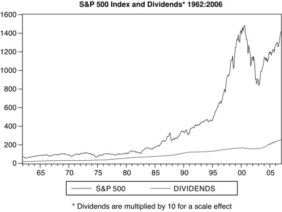
Before starting any analysis it is useful to examine the plot of the underlying time series variables. Figure 1 presents a plot of stock prices and dividends for the years 1962 through 2006. The stock prices are represented by the S&P 500 index and the dividends represent the dividend received by the owner of $1,000 worth of the S&P 500 index. The plot shows that the variables move together until the early 1980s. As a result of this visual analysis, we will entertain the possibility that the variables were cointegrated until the 1980s. After that, the common stochastic trend may have dissipated. We will first test for cointegration in the 1962–1982 period and then for the whole 1962–2006 period.
In accordance with the first step of the cointegration protocol, we must first establish the nonstationarity of the variables. To identify nonstationarity, we will use both formal and informal methods. The first informal test consists of analyzing the plot of the series shown in Figure 1. Neither series exhibits mean reversion. The dividend series wanders less from its mean than the stock prices. Nevertheless, neither series appears stationary.
The second informal method involves examining the autocorrelation function. We present in Table 1 the autocorrelation function for 36 lags of the S&P 500 index and the dividends for the 1962–2006 period using monthly data. The autocorrelations for the early lags are quite close to one. Furthermore, the autocorrelation function exhibits a slow decay at higher lags. This provides sufficient evidence to conclude that stock prices and dividends are nonstationary. When we inspect the autocorrelation function of their first differences (not shown), the autocorrelation of the first lag is not close to one. We may conclude the series are stationary in the first differences.
In Table 2, we present the results of formal tests of nonstationarity. The lag length for the ADF test was determined by the Schwarz criterion. The null hypothesis is that the S&P 500 stock index (dividends) contains a unit root; the alternative is that it does not. For both statistics, the ADF and the Phillips-Perron, the results indicate that the S&P 500 index is nonstationary and the changes in that index are stationary. The results for dividends are mixed. The ADF statistic supports the presence of a unit root in dividends, while the Phillips-Peron statistic does not. Since both the autocorrelation function and the ADF statistic conclude there is a unit root process, we shall presume that the dividend series is nonstationary. In sum, our analysis suggests that the S&P 500 index and dividends series each contain a stochastic trend in the levels, but not in their first differences.
In the next step of the protocol we examine whether the S&P 500 index and dividends are cointegrated. This is accomplished by estimating the long-run equilibrium relation by regressing the logarithm (log) of the S&P 500 index on the log of the dividends. We use the logarithms of both variables to help smooth the series. The results using monthly data are reported in Table 3 for both the 1962–1982 period and the 1962–2006 period. We pay little attention to the high t-statistic on the dividends variable because the t-test is not appropriate unless the variables are cointegrated. This is, of course, the issue.
Table 3 Cointegration Regression: S&P 500 and Dividends
Log S&P 500 = a + b log dividends + zt

Table 4 Augmented Dickey Fuller Tests of Residuals for Cointegration
Once we estimate the regression in step 2, the next step involves testing the residuals of the regression, zt, for stationarity. By definition, the residuals have a zero mean and lack a time trend. This simplifies the test for stationarity. This is accomplished by estimating equation (4). The null hypothesis is that the variables lack cointegration. If we conclude that p in equation (4) is significantly negative, then we reject the null hypothesis and conclude that the evidence is consistent with the presence of cointegration between the stock index and dividends. The appropriate lag lengths may be determined by the Akaike information criterion or theoretical and practical considerations. We decided to use a lag length of three periods representing one quarter. The results are presented in Table 4. For the 1962–1982 period, we may reject the null hypothesis of no cointegration at the 10% level of statistical significance. For the entire period (1962–2006), we cannot reject the null hypothesis (p = 0) of no cointegration. Apparently, the relationship between stock prices and dividends unraveled in the 1980s and the 1990s. This evidence is consistent with the existence of an Internet stock bubble in the 1990s.
Table 5 Error Correction Model: S&P 500 Index and Dividends 1962–1982

Having established that the S&P 500 index and dividends are cointegrated from 1962–1982, in the final step of the protocol we examine the interaction between stock prices and dividends by estimating the error-correction model, equations (5) and (6). It is useful at this point to review our interpretation of equations (5) and (6). Equation (5) claims that changes in the S&P 500 Index depend upon past changes in the S&P 500 Index and past changes in dividends and the extent of disequilibrium between the S&P 500 index and dividends. Equation (6) has a similar statistical interpretation. However, from a theoretical point of view, equation (6) is meaningless. Financial theory does not claim that changes in dividends are impacted either by past changes in stock prices or the extent of the disequilibrium between stock prices and dividends. As such, equation (6) degenerates into an autoregressive model of dividends.
We estimated the error-correction equations using three lags. The error term, zt−1, used in these error-correction regressions was obtained from OLS estimation of the cointegration equation reported in Table 3. Estimates of the error-correction equations are reported in Table 5. By construction, the error-correction term represents the degree to which the stock prices and dividends deviate from long-run equilibrium. The error-correction term is included in both equations to guarantee that the variables do not drift too far apart. If the variables are cointegrated, Engle and Granger (1987) showed that the coefficient on the error-correction term (yt−1 − axt−1) in at least one of the equations must be nonzero. The t value of the error-correction term in equation (5) is statistically different from zero. The coefficient of −0.07 is known as the speed of adjustment coefficient. It suggests that 7% of the previous month’s disequilibrium between the stock index and dividends is eliminated in the current month. In general, the higher the speed of adjustment coefficient, the faster the long-run equilibrium is restored. Since the speed of adjustment coefficient for the dividend equation is statistically indistinguishable from zero, all of the adjustment falls on the stock price.
An interesting observation from Table 5 relates to the lag structure of equation (5). The first lag on past stock price changes is statistically significant. This means that the change in the stock index this month depends upon the change during the last month. This is inconsistent with the efficient market hypothesis. On the other hand, the change in dividend lags is not statistically different from zero. The efficient market theory suggests, and the estimated equation confirms, that past changes in dividends do not affect the current changes in stock prices.
Johansen-Juselius Cointegration Tests
The Engle-Granger method does have some problems (see Enders, 1995). These problems are magnified in a multivariate (three or more variables) context. In principle, when the cointegrating equation is estimated (even in a two-variable problem), we may use any variable as the dependent variable. In our last example, this would entail placing dividends on the left-hand side of equation (2) and the S&P 500 index on the right-hand side. As the sample size approaches infinity, Engle and Granger (1987) showed the cointegration tests produce the same results irrespective of what variable you use as the dependent variable. The question then is: How large a sample is large enough?
A second problem is that the errors we use to test for cointegration are only estimates and not the true errors. Thus any mistakes made in estimating the error term, zt, in equation (2) are carried forward into the equation (3) regression. Finally, the Engle-Granger procedure is unable to detect multiple cointegrating relationships.
The procedures developed by Johansen and Juselius (1990) avoid these problems. Consider the following multivariate model:
where
ytis an n × 1 vector (y1t, y2t,… …ynt)’
ut
is an n-dimensional error term at t
Ais an n × n matrix of coefficients
If the variables display a time trend, we may wish to add the matrix A0 to equation (7). This would reflect a deterministic time trend. The same applies to equation (8) presented below. It does not change the nature of our analysis.
The model (without the deterministic time trend) can then be represented as:
Let B = I − A. I is the identity matrix of dimension n. The cointegration of the system is determined by the rank of B matrix. The highest rank of B one can obtain is n, the number of variables under consideration. If the rank of the matrix equals zero, then the B matrix is null. This means Δyt = 0+ ut, where 0 is the null vector. In this case yit will follow a random walk (yt = yt − 1 + ut) and no linear combination of yt will be stationary, so there are no cointegrating vectors.
If the rank of B is n, then each yit is an autoregressive process. This means each yit is stationary and thus they cannot be cointegrated. For any rank between 1 and n − 1, the system is cointegrated and the rank of the matrix is the number of cointegrating vectors.
The higher-order autoregressive representation is similar. Although it is more involved, the Johansen and Juselius estimation procedure can still handle it easily. Since the rank of a matrix equals the number of distinct nonzero characteristic roots of a matrix, the Johansen-Juselius procedure attempts to determine the number of nonzero characteristic roots of the relevant matrices. The procedure estimates the matrices and hence the characteristic roots with a maximum likelihood method.
The Johansen-Juselius procedure employs two statistics to test for nonzero characteristic roots. First they order the characteristic roots from high to low, λ1*> λ2*>… .λ>n*. λi* to estimate nonzero characteristic roots.
The first statistic, the trace test statistic, verifies the null hypothesis that at most i characteristic roots are different from zero. The alternative hypothesis is that more than i characteristic roots are nonzero. The statistic employed is:
(9) ![]()
where T is the number of included time periods. If all the characteristic roots are zero since ln(1) = 0, the statistic will equal zero. Thus low values of the test statistic will lead us to fail to reject the null hypothesis. The larger any characteristic root is, the more negative 1− λi* and the larger the test statistic and the more likely we will reject the null hypothesis.
The alternative test is called the maximum eigenvalue test since it is based on the largest eigenvalue. This statistic tests the null hypothesis that there are i cointegrating vectors against the alternative hypothesis of i + 1. This statistic is:
(10) ![]()
Again, if λi+1* = 0, then the test statistic will equal zero. So low (high) values of λi+1* will lead to a failure to reject (rejection of) the null hypothesis.
Johansen and Juselius derive critical values for both test statistics. The critical values are different if there is a deterministic time trend and an A0 matrix is included. Enders (1995) provides tables for both critical statistics with and without the trend terms. Software programs often provide critical values and the relevant p-values.
Testing of the Dynamic Relationships among Country Stock Markets
Many portfolio managers seek international diversification. If stock market returns in different countries were not highly correlated, then portfolio managers could obtain risk reduction without significant loss of return by investing in different countries. But with the advent of globalization and the simultaneous integration of capital markets, the risk-diversifying benefits of international investing have been subject to challenge. In this section, we illustrate how cointegration can shed light on this issue and apply the Johansen-Juselius technique.
The idea of a common currency for the European countries is to reduce transactions costs and more closely link the economies. We shall use cointegration to examine whether the stock markets of France, Germany, and the Netherlands are linked following the introduction of the Euro in 1999. We use monthly data for the period 1999–2006.
The first step to test for cointegration is to establish that the three stock indexes are nonstationary in the levels and stationary in the first differences. In testing the present value model, we presented the autocorrelation function (the ADF statistic), and the Phillips-Perron statistic. For reasons of space, we will not repeat this. Next we should establish the appropriate lag length for equation (8). This is typically done by estimating a traditional vector autoregressive (VAR) model and applying a multivariate version of the Akaike information criterion or Schwarz criterion. For our model, we use one lag, and thus the model takes the form:
(11) ![]()
where yt is the n × 3 vector (y1t, y2t, y3t)’ of the logs of the stock market index for France, Germany, and the Netherlands (i.e., element y1t is the log of the French index at time t; y2t is the log of the German index at time t; and y3t is the log of the Netherlands index at time t). We use logs of the stock market indexes to smooth the series. A0 and A1 are n × n matrices of parameters and ut is the n × n error matrix.
The next step is to estimate the model. This means fitting equation (8). We incorporated a linear time trend, hence the inclusion of the matrix A0. Since there are restrictions across the equations, the procedure uses a maximum likelihood estimation procedure and not OLS. The focus of this estimation is not on the parameters of the A matrices. Few software programs present these estimates; rather, the emphasis is on the characteristic roots of the matrix B, which are estimated to determine the rank of the matrix.
The estimates of the characteristic roots are presented in Table 6. We want to establish whether i indexes are cointegrated. Thus, we test the null hypothesis that the indexes lack cointegration. To accomplish this, the λtrace (0) statistic is calculated. Table 6 also provides this statistic. To ensure comprehension of this important statistic, we detail its calculation.
Table 6 Cointegration Test

We have 96 usable observations.

As reported in Table 6, this exceeds the critical value for 5% significance of 29.80 and has a p-value of 0.02. Thus, we may reject the null hypothesis at a 5% level of significance and conclude that the evidence is consistent with at least one cointegrating vector. Next we can examine λtrace (1) to test the null hypothesis of at most 1 cointegrating vector against the alternative of 2 cointegrating vectors. Table 6 shows that λ1 at 8.33 is less than the critical value of 15.49 necessary to establish statistical significance at the 5% level. We do not reject the null hypothesis. We therefore conclude that there is at least one cointegrating vector. There is no need to evaluate λtrace (2).
The λmax statistic reinforces our conclusion. We can use λmax (0, 1) to test the null hypothesis that the variables lack cointegration against the alternative that they are cointegrated with one cointegrating vector. Table 6 presents the value of λmax (0, 1). Again, for pedagogic reasons we outline the calculation of λmax (0, 1).
![]()
The computed value of 24.72 exceeds the critical value of 21.13 at the 5% significance level and has a p-value of 0.01. Once again, this leads us to reject the null hypothesis that the indexes lack cointegration and conclude that there exists at least one cointegrating vector.
Table 7 Cointegrating Equation and Error Correction Equations 1999–2007
Panel A: Cointegrating Equation
France 4.82 + 2.13 Germany -1.71 Netherlands
[-8.41] [5.25]
Panel B: Error Correction Equations

The next step requires a presentation of the cointegrating equation and an analysis of the error-correction model. Table 7 presents both. The cointegrating equation is a multivariate representation of zt−1 in the Engle-Granger method. This is presented in panel A of Table 7. The error-correction model takes the following representation.

The notation of equation (12) differs somewhat from the notation of equations (5) and (6). The notation used in equation (12) reflects the matrix notation adopted for the Johansen-Juselius method in equation (8). Nevertheless, for expositional convenience, we did not use the matrix notation for the error-correction term. Again, the Δ means the first difference of the variable; thus Δy1t−1 means the change in the log of the French stock index in period t − 1, (y1t−1 − y1t−2). Equation (12) claims that changes in the log of the French stock index are due to changes in the French stock index during the last two (2) periods; changes in the German stock index during the last two periods; changes in the Netherlands stock index during the last two periods; and finally deviations of the French stock index from its stochastic trend with Germany and the Netherlands. An analogous equation could be written for both Germany and the Netherlands.
Panel B of Table 7 presents the error-correction model estimates for each of the three countries. The software used a two-period lag for the past values of the changes in the stock indexes as indicated by the Schwarz criterion.
The error-correction term in each equation reflects the deviation from the long-run stochastic trend of that stock index in the last period. It should be noted that in contrast to the two-step procedure of the Engle-Granger approach, the Johansen-Juselius approach estimates the speed of adjustment coefficient in one step. It provides insight into the short-run dynamics. This coefficient is insignificant (at the 5% level) for Germany. This means that stock prices in Germany do not change in response to deviations from their stochastic trend with France and the Netherlands. Because the variables are cointegrated, we are guaranteed that at least one speed of adjustment coefficient will be significant. In fact, the speed of adjustment coefficients of both France and the Netherlands attain statistical significance (at the 5% level) and are about the same size. This shows that when the economies of France and the Netherlands deviate from the common stochastic trend, they adjust. In France about 15% and in the Netherlands about 17% of the last-period deviation is corrected during this period.
for France, neither past changes in its own stock index nor the past changes in Germany’s stock index appear to affect French stock prices. The changes in the lagged values of both indexes lack statistical significance. Only the second lag of the Netherlands stock index attained significance. For Germany, the past changes in its own stock prices and the past changes in the stock indexes of the other countries failed to obtain significance at the 5% level. For the Netherlands, its own second-period lag obtained statistical significance. Nevertheless, the failure of individual lags to obtain significance does not mean that jointly the lags are insignificant.
To see this, we turn to an examination of Granger causality in the error-correction models. Granger causality helps us to classify the variables into dependent and independent. A variable Granger causes another variable when past values of that variable improve our ability to forecast the original variable. To test for Granger causality, an F-test is employed to verify whether the lagged changes in, say, the stock index of France jointly zero in the German equation. Table 8 reports the results of pairwise Granger causality tests. We find that France and Germany do not Granger cause each other at any conventional levels of significance. The smaller Netherlands economy finds its stock prices Granger caused by both France and Germany but the Netherlands does not Granger cause either French or German stock prices at conventional levels of significance.
Table 8 Cointegration Test Results 1975–2000
Empirical Illustration of a Test for the Presence of a Housing Bubble
The third application demonstrates the use of cointegration to test the possibility of a bubble in the housing market. As we illustrated in our previous examples, the beginning of any analysis is a picture of the time series under examination. Figure 2 shows the trend in the U.S. housing index from 1975 to the third quarter of 2007. Clearly, since 2001 the United States has experienced several years of strong home price increases. Also, the figure illustrates that the rise began to slow in 2005. At this time we know that housing prices collapsed in 2008. This sort of evidence has led the financial and the general press to conclude that the U.S. housing market has experienced a bubble. However, the detection of a bubble after the fact is of little practical use. The question is, can cointegration provide evidence of a bubble before the bubble bursts?
Figure 2 Home Prices in the United States
*The bursting of a real estate bubble has important implications for the U.S. economy. Residential real estate is an important component of householder wealth. In 1996, it represented 39% of household wealth. This figure is reprinted from Arshanapalli and Nelson (2008) with the permission of the Institute for Business and Finance Research.

The widely accepted efficient market theory claims that financial asset prices reflect all the publicly available information at all times. This denies the possibility of a bubble. While some may believe prices are too high relative to fundamental factors, according to the theory they are wrong, because investors recognize immediately if the price of anything is too high (or too low) and respond by selling (or purchasing) the asset until the over-(under) pricing is eliminated. A mountainous body of academic research (see Fama, 1970, for a sampling) supports this view.
Nevertheless, the efficient market theory has been subject to much serious criticism (Shiller, 2003). Furthermore, much of the research focused on financial assets. The efficient market theory assumes that investors can sell an asset short to eliminate overpricing. Real estate is a real and illiquid asset. During the period of the housing price run-up there was no mechanism known to us for shorting a residential home. A futures market for housing is a relatively recent innovation. These markets do not function well enough to fulfill the assumptions of the efficient market theory. Thus, we should not dismiss the possibility of a housing bubble out of hand.
Arshanapalli and Nelson (2008) tested for the existence of a housing bubble, examining the stability of the underlying relationship of home prices and the economic forces that determine them. A relationship suddenly becomes unstable when rising home prices are not justified by the underlying economic fundamentals. Cointegration is well suited to test for this. Cointegration implies that two variables share a common stochastic trend. A common stochastic trend does not simply mean that they move upward or downward together, but rather that the variables may share both prolonged upward and prolonged downward movements.
Suppose housing prices are cointegrated with an economic variable and a bubble develops in the housing market, then housing prices rise without a corresponding rise in the variable. This implies the severing of a long-term relationship between housing prices and the variable. In other words, the cointegration should cease. In summary, if there were a housing bubble beginning in about 2000, then the variables, which were cointegrated with housing prices before 2000, will no longer remain cointegrated after 2000.
Data
Quarterly data are used and the study covers the period 1975Q1–2007Q2. We employ the U.S. Office of Federal Housing Enterprise Oversight (OFHEO) Home Price quarterly index to measure housing prices. The index is not seasonally adjusted.
Next, we consider a series of seven variables that reflect the fundamental economic forces determining housing prices. The most important of these is income. Case and Shiller (2003) conclude that in nonbubble markets income explains most of the rise in housing prices. We employ two separate measures of income. The first is the mean of the middle quintile of the income distribution, denoted as the Middle Fifth. Second, we use the mean of the highest quintile of the income distribution, denoted as the Top Fifth. This attempts to account for the possibility that the wealthiest segment of the population influences housing prices disproportionately because of their greater mobility. The U.S. Census Bureau, Historical Income Tables-Families (all races), and the National Association of Realtors provided these data.
The mortgage rate represents a strong influence on consumer demand for housing. We obtained the 30-year conventional mortgage rate (fixed rate, first mortgages) from the Board of Governors of the U.S. Federal Reserve System. The civilian unemployment rate measures the state of the economy. The U.S. Bureau of Labor Statistics provided the seasonally adjusted percentage of civilian unemployment. We converted the monthly data for both variables to quarterly data by a simple mean. The Homebuilders Stock Index provides an indication of the state of the housing market. A capitalization-weighted, price-level index of homebuilding stocks based on stocks included in the S&P 500 stock index was obtained from Merrill Lynch.
The final variables measure the ability of consumers to handle mortgage debt. The household debt ratio is the ratio of household credit market debt outstanding to annualized personal disposable income. The data also came from the Board of Governors of the U.S. Federal Reserve System. The Housing Affordability Index for all homebuyers (HAI) measures whether or not a typical family could qualify for a mortgage loan on a typical home, assuming a 20% down payment. We define a typical home as the national median-priced, existing single–family home as calculated by NAR. In its final form used here, the HAI is essentially “median family income divided by qualifying income.” The index is interpreted as follows: A value of 100 means that a family with the median family income (from the U.S. Bureau of the Census and NAR) has exactly enough income to qualify for a mortgage on a median-priced home. National Association of Realtors (NAR) provided the data. In this research, the monthly HAI values result from quarterly samples.2
Again, the first step in establishing cointegration is to test the variables for stationarity. To establish nonstationarity we employed the ADF (augmented Dickey Fuller) test and the Phillips-Peron test. Although we do not display the results here, we conclude all the variables are nonstationary.
Next, we examine whether home prices and the seven fundamental variables are cointegrated. This is accomplished by examining a cointegrating regression for each of the seven variables with home prices. Table 8 presents the results of these cointegration tests for the 1975Q1–2000Q4 period. The Trace Statistic Test shows that for three of the seven variables, top fifth, middle fifth, and the unemployment rate, we may reject the null hypothesis of no cointegration at a 5% level of significance. Furthermore, we may reject the null hypothesis of no cointegration at the 10% level of statistical significance for one additional variable, the Homebuilders stock index. Thus for the period preceding the runup in home prices there appears to have been a strong link between home prices and both the income variables and the unemployment rate and a marginal link with the Homebuilders Stock Index.
Table 9 presents the results of these cointegration tests for the period 1975–2007Q3. The trace tests indicate the eigenvalues are not statistically distinguishable from zero in any equation at the 5% level. However, the P-value for the middle fifth of income was .0502. Recognizing the belief that the bubble burst in late 2005, we did the cointegration test for the period 1975–2005Q2. The P-value (hypothesized no. of CE(s) = none) for home prices vs. middle fifth of income was 11%. (Although we did not display the results, we cannot reject the hypothesis of no cointegration for any of the other fundamental variables during this period. This suggests that in the post-2005 period the normal relationship between home prices and income was reasserting itself. This result suggests that the linkage between home prices and fundamental variables has been substantially reduced after 2000. The evidence is consistent with a real estate bubble.
Table 9 Cointegration Test Results for the Whole Period: 1975–2007Q3

KEY POINTS
- Many of the variables of interest to finance professionals are nonstationary.
- The relationships among them can be fruitfully analyzed if they share a common stochastic trend. A way of capturing this common stochastic trend is the application of cointegration.
- Cointegration analysis can reveal interesting long-run relationships between the variables.
- It is possible that cointegrating variables may deviate in the short run from their relationship, but the error correction model shows how these variables adjust to the long-run equilibrium.
- Cointegration analysis can reveal interesting short-run asset pricing adjustments.
- The error-correction models tend to have a better forecasting performance than simple vector autoregressive models.
- Cointegration analysis shows when fundamental long-run relationships are severed. This is consistent with the presence of an asset price bubble.
NOTES
1. For a summary of these criteria, see Chap-ter 12 in Focardi and Fabozzi (2004).
2. For more details on the exact calculation, go to www.realtor.org.
REFERENCES
Arshanapalli, B., and Doukas, J. (1993). International stock market linkage: Evidence from the pre and post October 1987 period. Journal of Banking and Finance 17: 193–208.
Arshanapalli, B., and Nelson, W. (2008). A cointegration test to verify the housing bubble. The International Journal of Business and Finance Research 2: 35–44.
Case, K., and Shiller, R. (2003). Is there a bubble in the housing market. Brooking Papers on Economic Activities 2: 299–362.
Dickey, D., and Fuller, W. A. (1979). Distribution of the estimates for autoregressive time series with a unit root. Journal of the American Statistical Association 74: 427–431.
Dickey, D., and Fuller, W. A. (1981). Likelihood ratio statistics for autoregressive time series with a unit root. Econometrica 49: 427–431.
Enders, W. (1988). ARIMA and cointegration tests of purchasing power parity. Review of Economics and Statistics 70: 504–508.
Enders, W. (1995). Applied Econometric Time Series. Hoboken, NJ: Wiley.
Engle, R. F., and Granger, C. W. J. (1987). Cointegration and error-correction: Representation, estimation and testing. Econometrica 55: 251–276.
Engle, R. F., and Yoo, S. (1987). Forecasting and testing in co-integrated systems. Journal of Econometrics 35: 143–159.
Focardi, S. M., and Fabozzi, F. J. (2004). The Mathematics of Financial Modeling and Investment Management. Hoboken, NJ: John Wiley & Sons.
Gurkaynak, R. (2005). Econometric tests of asset price bubbles: Taking stock. Finance and Economics Discussion Series, Federal Reserve Board. Washington, D.C.
Hendry, D., and Juselius, K. (2000). Explaining cointegration analysis: Part II. Discussion Papers, University of Copenhagen, Department of Economics.
Johansen, S., and Juselius, K. (1990). Maximum likelihood estimation and inference on cointegration with application to the demand for money. Oxford Bulletin of Economics and Statistics 52: 169–209.
Liu, P., and Maddala, G. (1992). Using survey data to market efficiency in the foreign exchange market. Empirical Economics, 17: 303–314.
Phillips, P., and Perron, P. (1988). Testing for a unit root in time series regression. Biometrica 75: 335–346.
Shiller, R. (2003). From efficient markets theory to behavioral finance. Journal of Economic Perspectives 17: 83–104.
Stock, J., and Watson, M. (2003). Introduction to Econometrics. New York: Addison Wesley.