
Continuous Probability Distributions
In this entry, we introduce the concept of con-tinuous probability distributions. We present the continuous distribution function with its corresponding density function, a function unique to continuous probability laws. In this entry, parameters of location and scale such as the mean and higher moments—variance and skewness—are defined. For a more technical discussion of continuous distributions, see Evans, Hastings, and Peacock (2000) or Johnson, Kotz, and Balakrishnan(1995).
CONTINUOUS PROBABILITY DISTRIBUTION DESCRIBED
Suppose we are interested in outcomes that are no longer countable. Examples of such outcomes in finance are daily logarithmic stock returns, bond yields, and exchange rates. Technically, without limitations caused by rounding to a certain number of digits, we could imagine that any real number could provide a feasible outcome for the daily logarithmic return of some stock. That is, theset of feasible values that the outcomes are drawn from (i.e., the space Ω) is uncountable. The events are described by continuous intervals such as, for example, (−0.05, 0.05], which, referring to our example with daily logarithmic returns, would represent the event that the return at a given observation is more than −5% and at most 5%.
In the context of continuous probability distributions, we have the real numbers ![]() as the uncountable space Ω. The set of events is given by the Borel σ-algebra
as the uncountable space Ω. The set of events is given by the Borel σ-algebra ![]() , which is based on the half-open intervals of the form (
, which is based on the half-open intervals of the form (![]() ], for any real a. The space
], for any real a. The space ![]() and the σ-algebra
and the σ-algebra ![]() form the measurable space
form the measurable space ![]() , which we are to deal with throughout
this entry.
, which we are to deal with throughout
this entry.
DISTRIBUTION FUNCTION
To be able to assign a probability to an event in a unique way, in the context of continuous distributions we introduce as a device the continuous distribution function F(a), which expresses the probability that some event of the sort (![]() , a] occurs (i.e., that a number is realized that is at most a). (Formally, an outcome
, a] occurs (i.e., that a number is realized that is at most a). (Formally, an outcome ![]() is realized that lies inside of the interval (
is realized that lies inside of the interval (![]() ].) As with discrete random variables, this function is also referred to as the cumulative distribution function (cdf) since it aggregates the probability up to a certain value.
].) As with discrete random variables, this function is also referred to as the cumulative distribution function (cdf) since it aggregates the probability up to a certain value.
To relate to our previous example of daily logarithmic returns, the distribution function evaluated at say 0.05, that is, F(0.05), states the probability of some return of at most 5%. (The distribution function F is also referred to as the cumulative probability distribution function (often abbreviated cdf) expressing that the probability is given for the accumulation of all outcomes less than or equal to a certain value.)
For values x approaching ![]() , F tends to zero, while for values x approaching
, F tends to zero, while for values x approaching ![]() , F goes to 1. In between, F is monotonically increasing and right-continuous. More concisely, we list these properties below:
, F goes to 1. In between, F is monotonically increasing and right-continuous. More concisely, we list these properties below:

The behavior in the extremes—that is when x goes to either ![]() or
or ![]() —is provided by properties 1 and 2, respectively. Property 3 states that F should be monotonically increasing (i.e., never become less for increasing values). Finally, property 4 guarantees that F is right-continuous.
—is provided by properties 1 and 2, respectively. Property 3 states that F should be monotonically increasing (i.e., never become less for increasing values). Finally, property 4 guarantees that F is right-continuous.
Let us consider in detail the case when F(x) is a continuous distribution, that is, the distribution has no jumps. The continuous probability distribution function F is associated with the probability measure P through the relationship
![]()
that is, that values up to a occur, and
Therefore, from equation (1) we can see that the probability of some event related to an interval is given by the difference between the value of F at the upper bound b of the interval minus the value of F at the lower bound a. That is, the entire probability that an outcome of at most a occurs is subtracted from the greater event that an outcome of at most b occurs. Using set operations, we can express this as
![]()
For example as we have seen, the event of a daily return of more than −5% and, at most, 5% is given by (−0.05, 0.05]. So, the probability associated with this event is given by P((−0.05, 0.05]) = F(0.05) − F(−0.05).
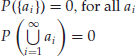
In contrast to a discrete probability distribution, a continuous probability distribution always assigns zero probability to countable events such as individual outcomes ai or unions thereof such as
![]()
That is,
From equation (2), we can apply the left-hand side of equation (1) also to events of the form (a,b) to obtain
Thus, it is irrelevant whether we state the probability of the daily logarithmic return being more than −5% and at most 5%, or the probability of the logarithmic return being more than −5% and less than 5%. They are the same because the probability of achieving a return of exactly 5% is zero. With a space Ω consisting of uncountably many possible values such as the set of real numbers, for example, each individual outcome is unlikely to occur. So, from a probabilistic point of view, one should never bet on an exact return or, associated with it, one particular stock price.
Since countable sets produce zero probability from a continuous probability measure, they belong to the so-called P-null sets. All events associated with P-null sets are unlikely events.
So, how do we assign probabilities to events in a continuous environment? The answer is given by equation (3). That, however, presumes knowledge of the distribution function F. The next task is to define the continuous distribution function F more specifically as explained next.
DENSITY FUNCTION
The continuous distribution function F of a probability measure P on (![]() ) is defined as follows
) is defined as follows

where f(t) is the density function of the probability measure P.
We interpret equation (4) as follows. Since, at any real value x the distribution function uniquely equals the probability that an outcome of at most x is realized, that is, F(x) = P((![]() ]), equation (4) states that this probability is obtained by integrating some function f over the interval from
]), equation (4) states that this probability is obtained by integrating some function f over the interval from ![]() up to the value x.
up to the value x.
What is the interpretation of this function f? The function f is the marginal rate of growth of the distribution function F at some point x. We know that with continuous distribution functions, the probability of exactly a value of x occurring is zero. However, the probability of observing a value inside of the interval between x and some very small step to the right Δx (i.e., [x, x + Δx)) is not necessarily zero. Between x and x + Δx, the distribution function F increases by exactly this probability; that is, the increment is
Now, if we divide F (x + Δx) − F(x) from equation (5) by the width of the interval Δx, we obtain the average probability or average increment of F per unit step on this interval. If we reduce the step size Δx to an infinitesimally small step ![]() , this average approaches the marginal rate of growth of F at x, which we denote f; that is,1
, this average approaches the marginal rate of growth of F at x, which we denote f; that is,1
At this point, let us recall the histogram with relative frequency density for class data. Over each class, the height of the histogram is given by the density of the class divided by the width of the corresponding class. Equation (6) is somewhat similar if we think of it this way. We divide the probability that some realization should be inside of the small interval. And, by letting the interval shrink to width zero, we obtain the marginal rate of growth or, equivalently, the derivative of F. (We assume that F is continuous and that the derivative of F exists.) Hence, we call f the probability density function or simply the density function. Commonly, it is abbreviated as pdf.
Now, when we refocus on equation (4), we see that the probability of some occurrence of at most x is given by integration of the density function f over the interval (![]() ]. Again, there is an analogy to the histogram. The relative frequency of some class is given by the density multiplied by the corresponding class width. With continuous probability distributions, at each value t, we multiply the corresponding density f(t) by the infinitesimally small interval width dt. Finally, we integrate all values of f (weighted by dt) up to x to obtain the probability for (
]. Again, there is an analogy to the histogram. The relative frequency of some class is given by the density multiplied by the corresponding class width. With continuous probability distributions, at each value t, we multiply the corresponding density f(t) by the infinitesimally small interval width dt. Finally, we integrate all values of f (weighted by dt) up to x to obtain the probability for (![]() ]. This, again, is similar to histograms: In order to obtain the cumulative relative frequency at some value x, we compute the area covered by the histogram up to value x.
]. This, again, is similar to histograms: In order to obtain the cumulative relative frequency at some value x, we compute the area covered by the histogram up to value x.
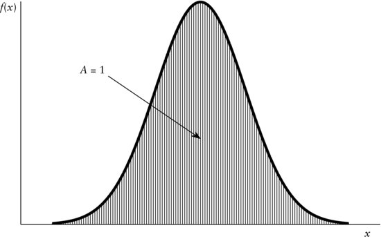
In Figure 1, we compare the histogram and the probability density function. The histogram with density h is indicated by the dotted lines while the density function f is given by the solid line. We can now see how the probability ![]() is derived through integrating the marginal rate f over the interval
is derived through integrating the marginal rate f over the interval ![]() with respect to the values t. The resulting total probability is then given by the area A1 of the example in Figure 1. This is analogous to class data where we would tally the areas of the rectangles whose upper bounds are less than
with respect to the values t. The resulting total probability is then given by the area A1 of the example in Figure 1. This is analogous to class data where we would tally the areas of the rectangles whose upper bounds are less than ![]() and the part of the area of the rectangle containing
and the part of the area of the rectangle containing ![]() up to the dash-dotted vertical line.
up to the dash-dotted vertical line.
Figure 1 Comparison of Histogram and Density Function
Note: Area A1 represents probability P((![]() ]) derived through integration of f(t) with respect to t between
]) derived through integration of f(t) with respect to t between ![]() and
and ![]()

Requirements on the Density Function
Given the uncountable space ![]() (i.e., the real numbers) and the corresponding set of events given by the Borel σ-algebra
(i.e., the real numbers) and the corresponding set of events given by the Borel σ-algebra ![]() , we can give a more rigorous formal definition of the density function. The density function f of probability measure P on the measurable space (
, we can give a more rigorous formal definition of the density function. The density function f of probability measure P on the measurable space (![]() ) with distributionfunction F is a Borel-measurable function f satisfying.
) with distributionfunction F is a Borel-measurable function f satisfying.

with ![]() for all
for all ![]() and
and

By the requirement of Borel-measurability, we simply assume that the real-valued images generated by f have their origins in the Borel σ-algebra ![]() . Informally, for any value y = f(t), we can trace the corresponding origin(s) t in
. Informally, for any value y = f(t), we can trace the corresponding origin(s) t in ![]() that is (are) mapped to y through the function f. Otherwise, we might incur problems computing the integral in equation (7) for reasons that are beyond the scope of this entry.
that is (are) mapped to y through the function f. Otherwise, we might incur problems computing the integral in equation (7) for reasons that are beyond the scope of this entry.
From definition of the density function given by equation (7), we see that it is reasonable that f be a function that exclusively assumes nonnegative values. Although we have not mentioned this so far, it is immediately intuitive since f is the marginal rate of growth of the continuous distribution function F. At each t, f(t) · dt represents the limit probability that a value inside of the interval (t, t + dt] should occur, which can never be negative. Moreover, we require the integration of f over the entire domain from ![]() to
to ![]() to yield 1, which is intuitively reasonable since this integral gives the probability that any real value occurs.
to yield 1, which is intuitively reasonable since this integral gives the probability that any real value occurs.
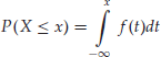
The requirement

implies the graphical interpretation that the area enclosed between the graph of f over the entire interval (![]() ) and the horizontal axis equals one. This is displayed in Figure 2 by the shaded area A. For example, to visualize graphically what is meant by
) and the horizontal axis equals one. This is displayed in Figure 2 by the shaded area A. For example, to visualize graphically what is meant by
Figure 2 Graphical Interpretation of the Equality ![]()

in equation (7), we can use Figure 1. Suppose the value x were located at the intersection of the vertical dash-dotted line and the horizontal axis (i.e., ![]() ). Then, the shaded area A1 represents the value of the integral and, therefore, the probability of occurrence of a value of at most x. To interpret
). Then, the shaded area A1 represents the value of the integral and, therefore, the probability of occurrence of a value of at most x. To interpret

graphically, look at Figure 3. The area representing the value of the interval is indicated by A. So, the probability of some occurrence of at least a and at most b is given by A. Here again, the resemblance to the histogram becomes obvious in that we divide one area above some class, for example, by the total area, and this ratio equates the according relative frequency.
Figure 3 Graphical Interpretation of ![]()

For the sake of completeness, it should be mentioned without indulging in the reasoning behind it that there are probability measures P on (![]() ) even with continuous distribution functions that do not have density functions as defined in equation (7). But, in our context, we will only regard probability measures with continuous distribution functions with associated density functions so that the equalities of equation (7) are fulfilled.
) even with continuous distribution functions that do not have density functions as defined in equation (7). But, in our context, we will only regard probability measures with continuous distribution functions with associated density functions so that the equalities of equation (7) are fulfilled.
Sometimes, alternative representations equivalent to equation (7) are used. Typically, the following expressions are used

Note that in the first two equalities, (8a) and (8b), the indicator function ![]() is used. The last two equalities, (8c) and (8d), can be used even if there is no density function and, therefore, are of a more general form. We will, however, predominantly apply the representation given by equation (7) and occasionally resort to the last two forms above.
is used. The last two equalities, (8c) and (8d), can be used even if there is no density function and, therefore, are of a more general form. We will, however, predominantly apply the representation given by equation (7) and occasionally resort to the last two forms above.
We introduce the term support at this point to refer to the part of the real line where the density is truly positive, that is, all those x where f(x) > 0.
CONTINUOUS RANDOM VARIABLE
So far, we have only considered continuous probability distributions and densities. We yet have to introduce the quantity of greatest interest to us in this entry, the continuous random variable. For example, stock returns, bond yields, and exchange rates are usually modeled as continuous random variables.
Informally stated, a continuous random variable assumes certain values governed by a probability law uniquely linked to a continuous distribution function F. Consequently, it has a density function associated with its distribution. Often, the random variable is merely described by its density function rather than the probability law or the distribution function.
By convention, let us indicate the random variables by capital letters. Recall that any random variable, and in particular a continuous random variable X, is a measurable function. Let us assume that X is a function from the probability space ![]() into the state space
into the state space ![]() . That is, origin and image space coincide. The corresponding σ-algebrae containing events of the elementary outcomes ω and the events in the image space X(ω), respectively, are both given by the Borel σ-algebra
. That is, origin and image space coincide. The corresponding σ-algebrae containing events of the elementary outcomes ω and the events in the image space X(ω), respectively, are both given by the Borel σ-algebra ![]() . Now, we can be more specific by requiring the continuous random variable X to be a
. Now, we can be more specific by requiring the continuous random variable X to be a ![]() −
− ![]() –measurable real-valued function. That implies, for example, that any event
–measurable real-valued function. That implies, for example, that any event ![]() , which is in
, which is in ![]() , has its origin X−1((a,b]) in
, has its origin X−1((a,b]) in ![]() , as well. Measur-ability is important when we want to derive the probability of events in the state space such as
, as well. Measur-ability is important when we want to derive the probability of events in the state space such as ![]() from original events in the probability space such as
from original events in the probability space such as ![]() . At this point, one should not be concerned that the theory is somewhat overwhelming. It will become easier to understand once we move to the examples.
. At this point, one should not be concerned that the theory is somewhat overwhelming. It will become easier to understand once we move to the examples.
COMPUTING PROBABILITIES FROM THE DENSITY FUNCTION
The relationship between the continuous random variable X and its density is given by the following.2 Suppose X has density f, then the probability of some event ![]() is computed as
is computed as

which is equivalent to F(x) and F(b) − F(a) respectively, because of the one-to-one relationship between the density f and the distribution function F of X.
As explained earlier, using indicator functions, equation (9) could be alternatively written as

In the following, we will introduce parameters of location and spread such as the mean and the variance, for example. In contrast to the data-dependent statistics, parameters of random variables never change. Some probability distributions can be sufficiently described by their parameters. They are referred to as parametric distributions. For example, for the normal distribution we introduce shortly, it is sufficient to know the parameters mean and variance to completely determine the corresponding distribution function. That is, the shape of parametric distributions is governed only by the respective parameters.
LOCATION PARAMETERS
The most important location parameter is the mean that is also referred to as the first moment. It is the only location parameter presented in this entry.
The mean can be thought of as an average value. It is the number that one would have to expect for some random variable X with given density function f. The mean is defined as follows: Let X be a real-valued random variable on the space ![]() with Borel σ-algebra
with Borel σ-algebra ![]() . The mean is given by
. The mean is given by

in case the integral on the right-hand side of equation (10) exists (i.e., is finite). Typically, the mean parameter is denoted as μ.
In equation (10) that defines the mean, we weight each possible value x that the random variable X might assume by the product of the density at this value, f(x), and step size dx. Recall that the product f(x) · dx can be thought of as the limiting probability of attaining the value x. Finally, the mean is given as the integral over these weighted values. Thus, equation (10) is similarly understood as the definition of the mean of a discrete random variable where, instead of integrated, the probability-weighted values are summed.
DISPERSION PARAMETERS
We turn our focus toward measures of spread or, in other words, dispersion measures. Again, as with the previously introduced measures of location, in probability theory the dispersion measures are universally given parameters. Here, we introduce the moments of higher order, variance, standard deviation, and the skewness parameters.
Moments of Higher Order
It might sometimes be necessary to compute moments of higher order. As we already know from descriptive statistics, the mean is the moment of order one. (Alternatively, we often say the first moment. For the higher orders k, we consequently might refer to the k-th moment.) However, one might not be interested in the expected value of some quantity itself but of its square. If we treat this quantity as a continuous random variable, we compute what is the second moment.
Let X be a real-valued random variable on the space ![]() with Borel σ-algebra
with Borel σ-algebra ![]() . The moment of order k is given by the expression
. The moment of order k is given by the expression

in case the integral on the right-hand side of equation (11) exists (i.e., is finite).
From equation (11), we learn that higher-order moments are equivalent to simply computing the mean of X taken to the k-th power.
Variance
The variance involves computing the expected squared deviation from the mean E(X) = μ of some random variable X. For a continuous random variable X, the variance is defined as follows: Let X be a real-valued random variable on the space ![]() with Borel σ-algebra
with Borel σ-algebra ![]() , then the variance is
, then the variance is

in case the integral on the right-hand side of equation (12) exists (i.e., is finite). Often, the variance in equation (12) is denoted by the symbol σ2.
In equation (12), at each value x, we square the deviation from the mean and weight it by the density at x times the step size dx. The latter product, again, can be viewed as the limiting probability of the random variable X assuming the value x. The square inflates large deviations even more compared to smaller ones. For some random variable to have a small variance, it is essential to have a quickly vanishing density in the parts where the deviations (x − μ) become large.
All distributions that we discuss in this entry are parametric distributions. For some of them, it is enough to know the mean μ and variance σ2 and consequently, we will resort to these two parameters often. Historically, the variance has often been given the role of risk measure in context of portfolio theory. Suppose we have two random variables R1 and R2 representing the returns of two stocks, S1 and S2, with equal means ![]() and
and ![]() , respectively, so that
, respectively, so that ![]() . Moreover, let R1 and R2 have variances
. Moreover, let R1 and R2 have variances ![]() and
and ![]() , respectively, with
, respectively, with ![]() . Then, omitting further theory, at this moment, we prefer S1 to S2 because of the S1's smaller variance. We demonstrate this in Figure 4. The dashed line represents the graph of the first density function while the second one is depicted by the solid line. Both density functions yield the same mean (i.e.,
. Then, omitting further theory, at this moment, we prefer S1 to S2 because of the S1's smaller variance. We demonstrate this in Figure 4. The dashed line represents the graph of the first density function while the second one is depicted by the solid line. Both density functions yield the same mean (i.e., ![]() ). However, the variance from the first density function, given by the dashed graph, is smaller than that of the solid graph (i.e.,
). However, the variance from the first density function, given by the dashed graph, is smaller than that of the solid graph (i.e., ![]() ). Thus, using variance as the risk measure and resorting to density functions that can be sufficiently described by the mean and variance, we can state that density function for S1 (dashed graph) is preferable. We can interpret the figure as follows.
). Thus, using variance as the risk measure and resorting to density functions that can be sufficiently described by the mean and variance, we can state that density function for S1 (dashed graph) is preferable. We can interpret the figure as follows.
Figure 4 Two Density Functions Yielding Common Means, μ1 = μ2, but Different Variances, ![]()
Note: Dashed graph: ![]() . Solid graph:
. Solid graph: ![]() .
.
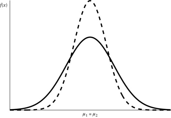
Since the variance of the distribution with the dashed density graph is smaller, the probability mass is less dispersed over all x values. Hence, the density is more condensed about the center and more quickly vanishing in the extreme left and right ends, the so-called tails. On the other hand, the second distribution with the solid density graph has a larger variance, which can be verified by the overall flatter and more expanded density function. About the center, it is lower and less compressed than the dashed density graph, implying that the second distribution assigns less probability to events immediately near the center. However, the density function of the second distribution decays more slowly in the tails than the first, which means that under the governance of the latter, extreme events are less likely than under the second probability law.
Standard Deviation
The parameter related to the variance is the standard deviation. As we know from descriptive statistics described earlier in this book, the standard deviation is the positive square root of the variance. That is, let X be a real-valued random variable on the space ![]() with Borel σ-algebra
with Borel σ-algebra ![]() . Furthermore, let its mean and variance be given by μ and σ2, respectively. The standard deviation is defined as
. Furthermore, let its mean and variance be given by μ and σ2, respectively. The standard deviation is defined as
![]()
For example, in the context of stock returns, one often expresses using the standard deviation the return's fluctuation around its mean. The standard deviation is often more appealing than the variance since the latter uses squares, which are a different scale from the original values of X. Even though mathematically not quite correct, the standard deviation, denoted by σ, is commonly interpreted as the average deviation from the mean.
Skewness
Consider the density function portrayed in Figure 5. The figure is obviously symmetric about some location parameter μ in the sense that ![]() . Suppose instead that we encounter a density function f of some random variable X that is depicted in Figure 6. This figure is not symmetric about any location parameter. Consequently, some quantity stating the extent to which the density function is deviating from symmetry is needed. This is accomplished by a parameter referred to as skewness. This parameter measures the degree to which the density function leans to either side, if at all.
. Suppose instead that we encounter a density function f of some random variable X that is depicted in Figure 6. This figure is not symmetric about any location parameter. Consequently, some quantity stating the extent to which the density function is deviating from symmetry is needed. This is accomplished by a parameter referred to as skewness. This parameter measures the degree to which the density function leans to either side, if at all.
Figure 5 Example of Some Symmetric Density Function f(x)

Figure 6 Example of Some Asymmetric Density Function f(x)

Let X be a real-valued random variable on the space ![]() with Borel σ-algebra
with Borel σ-algebra ![]() , variance σ2, and mean μ = E(X). The skewness parameter, denoted by γ, is given by
, variance σ2, and mean μ = E(X). The skewness parameter, denoted by γ, is given by
![]()
The skewness measure given above is referred to as the Pearson skewness measure. Negative values indicate skewness to the left (i.e., left skewed) while skewness to the right is given by positive values (i.e., right skewed).
The design of the skewness parameter follows the following reasoning. In the numerator, we measure the distance from every value x to the mean E(X) of random variable X. To overweight larger deviations, we take them to a higher power than one. In contrast to the variance where we use squares, in the case of skewness we take the third power since three is an odd number and thereby preserves both the signs and directions ofthe deviations. Due to this sign preservation, symmetric density functions yield zero skewness since all deviations to the left of the mean cancel their counterparts to the right. To standardize the deviations, we scale them by dividing by the standard deviation, also taken to the third power. So, the skewness parameter is not influenced by the standard deviation of the distributions. If we did not scale the skewness parameter in this way, distribution functions with density functions having large variances would always produce larger skewness even though the density is not really tilted more pronouncedly than some similar density with smaller variance.
We graphically illustrate the skewness parameter γ in Figure 6 for some density function f(x). A density function f that assumes positive values f(x) only for positive real values (i.e., x > 0) but zero for ![]() is shown in the figure. The random variable X with density function f has mean μ = 1.65. Its standard deviation is computed as σ = 0.957. The value of the skewness parameter is γ = 0.7224, indicating a positive skewness. The sign of the skewness parameter can be easily verified by analyzing the density graph. The density peaks just a little to the right of the leftmost value x = 0. Toward the left tail, the density decays abruptly and vanishes at zero. Toward the right tail, things look very different in that f decays very slowly, approaching a level of f = 0 as x goes to positive infinity. (The graph is depicted for
is shown in the figure. The random variable X with density function f has mean μ = 1.65. Its standard deviation is computed as σ = 0.957. The value of the skewness parameter is γ = 0.7224, indicating a positive skewness. The sign of the skewness parameter can be easily verified by analyzing the density graph. The density peaks just a little to the right of the leftmost value x = 0. Toward the left tail, the density decays abruptly and vanishes at zero. Toward the right tail, things look very different in that f decays very slowly, approaching a level of f = 0 as x goes to positive infinity. (The graph is depicted for ![]() .)
.)
KEY POINTS
- A continuous random variable is a random variable that does not only assume values from a set of discrete values but may assume any real value from within one or more intervals. Often, asset returns are modeled as continuous random variables.
- The continuous distribution function is the probability distribution associated with a continuous random variable. It distinguishes itself from the discrete probability distribution in that it gives positive probability only to entire intervals rather than some discrete values only.
- To appreciate continuous random variables, it is necessary to understand the concept of the derivative of some function, which is the marginal rate of growth of some function at a certain point. It can be conceived as the slope of the function at some point considering only very small increments in the argument of the function away from the point.
- The density function determines how the probability mass of one is distributed across the real line. Hence, it would be counterintuitive if that function were ever negative such that we require it to be nonnegative. Technically, it is the marginal rate of growth of the distribution function at any position or, in other words, its derivative.
- As support of some probability distribution, we define the subset of the real numbers that represents 100% of the probability. For the continuous probability distributions, it is the collection of intervals where the associated probability density is positive.
NOTES
1. The expression ![]() is equivalent to the increment F(x + Δx) − F(x) as Δx goes to zero.
is equivalent to the increment F(x + Δx) − F(x) as Δx goes to zero.
2. Sometimes the density of X is explicitly indexed fx. We will not do so here, however, except where we believe not doing so will lead to confusion. The same holds for its distribution function F.
REFERENCES
Evans, M., Hastings, N., and Peacock, B. (2000). Statistical Distributions, 3rd ed. New York: Wiley.
Johnson, N. L., Kotz, S., and Balakrishnan, N. (1995). Continuous Univariate Distributions, vol. 2, 2nd ed. New York: Wiley.